Downloaded 12 times

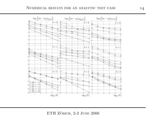
![Numerical results for an analytic test case
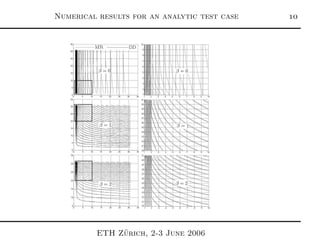
Ω =]0, 1[2
, ΓD = Ø
Parameters α > 0, β > 0,
Right hand side: f (y, x) ≡ yα
α2
− 1
xβ
y2
+ β(β − 1)xβ−2
Neumann datum:
g(x, y) = α if y = 1, −βyα
xβ−1
if x = 0, βyα
if x = 1.
Solution: u(x, y) ≡ yα
xβ
.
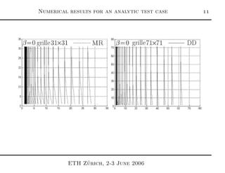
Comparison between
the present method (DD)
the use of classical P1 finite elements (MR)
ETH Z¨urich, 2-3 June 2006](https://image.slidesharecdn.com/slidesefef-150310030533-conversion-gate01/85/A-new-axisymmetric-finite-element-9-320.jpg)

This document summarizes a presentation on developing a natural finite element for axisymmetric problems. It introduces an axisymmetric model problem, defines appropriate axisymmetric Sobolev spaces, and presents a discrete formulation using a P1 finite element on triangles. Numerical results on a test problem show the method achieves the same convergence rates as classical approaches but with significantly smaller errors. The analysis draws on previous work to prove first-order approximation properties under certain mesh assumptions.


