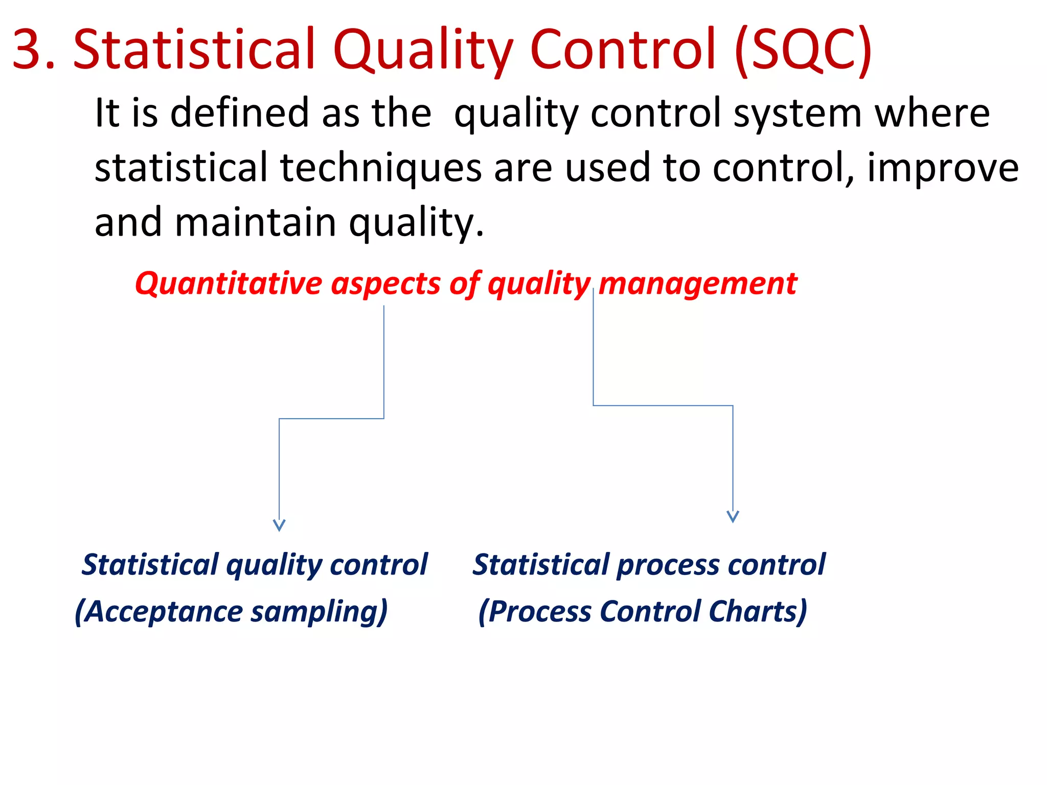
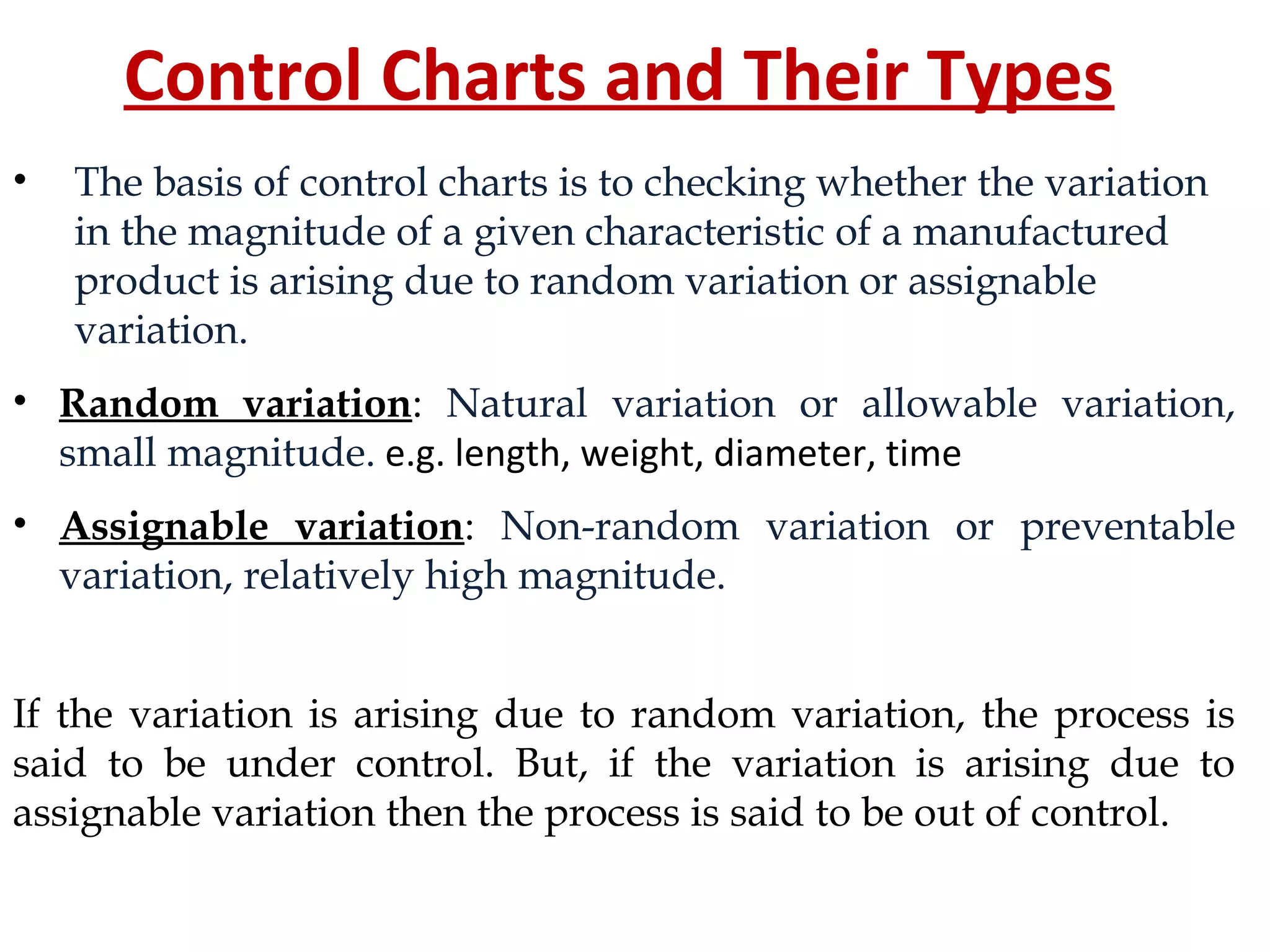
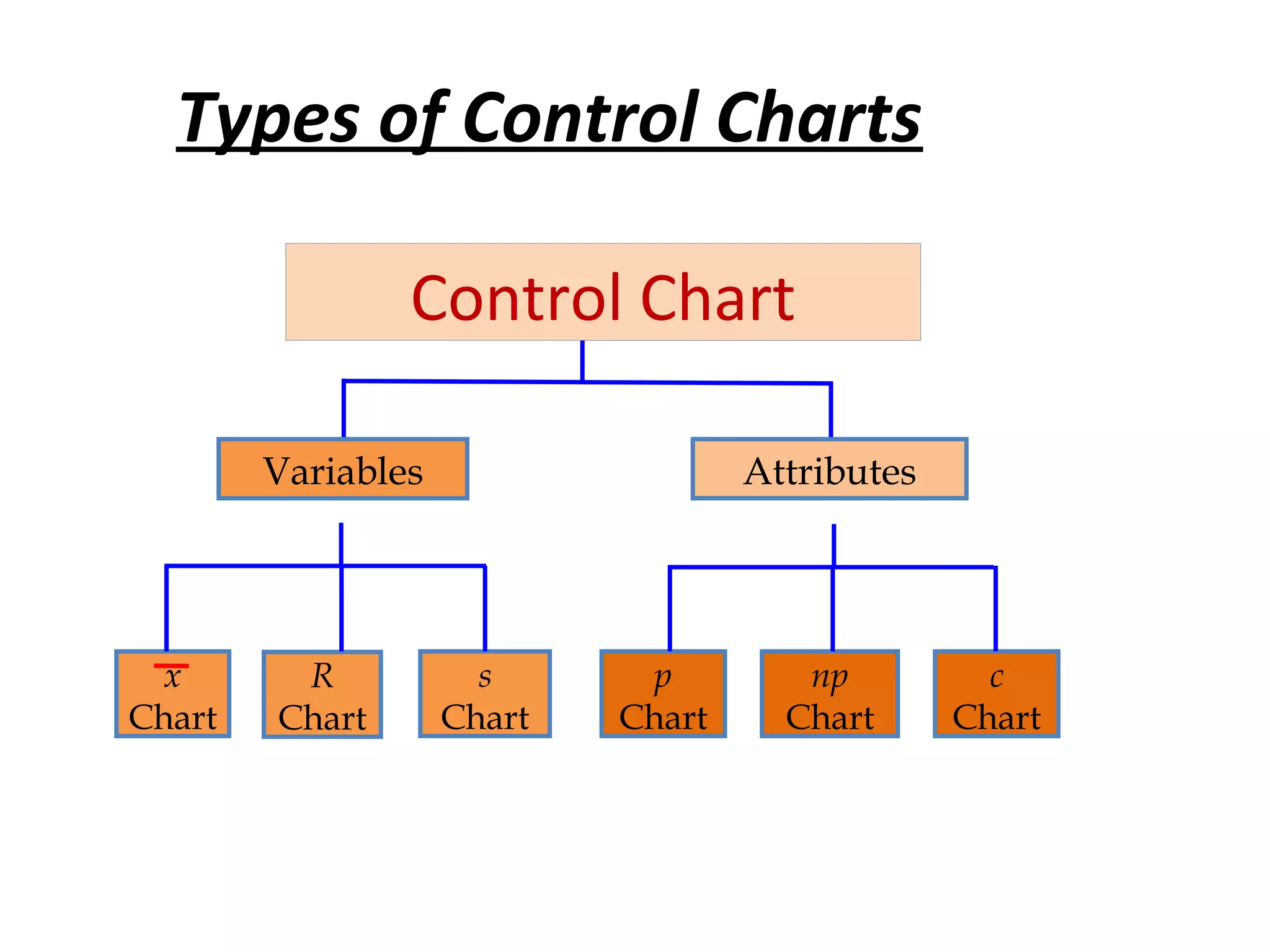
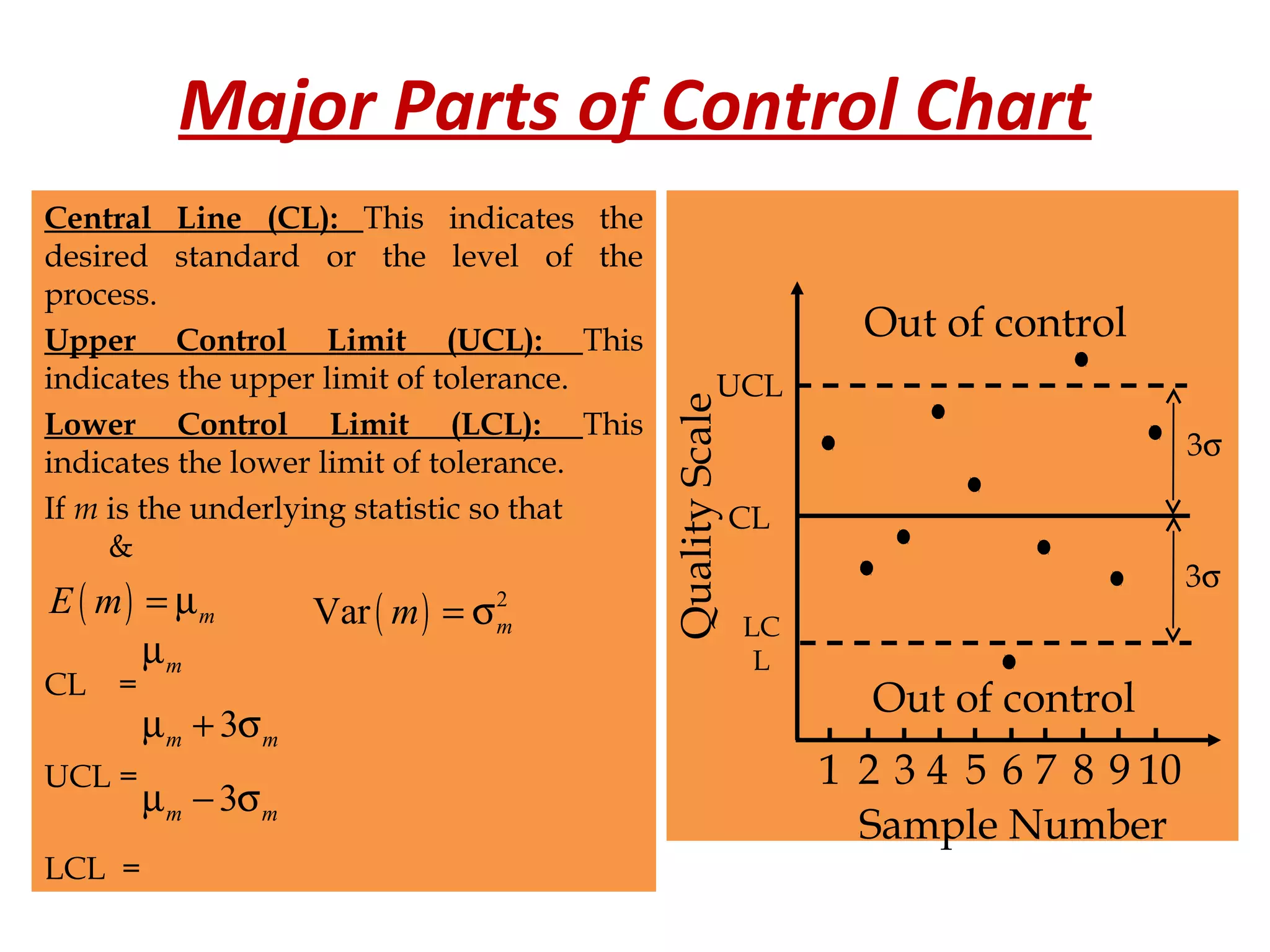
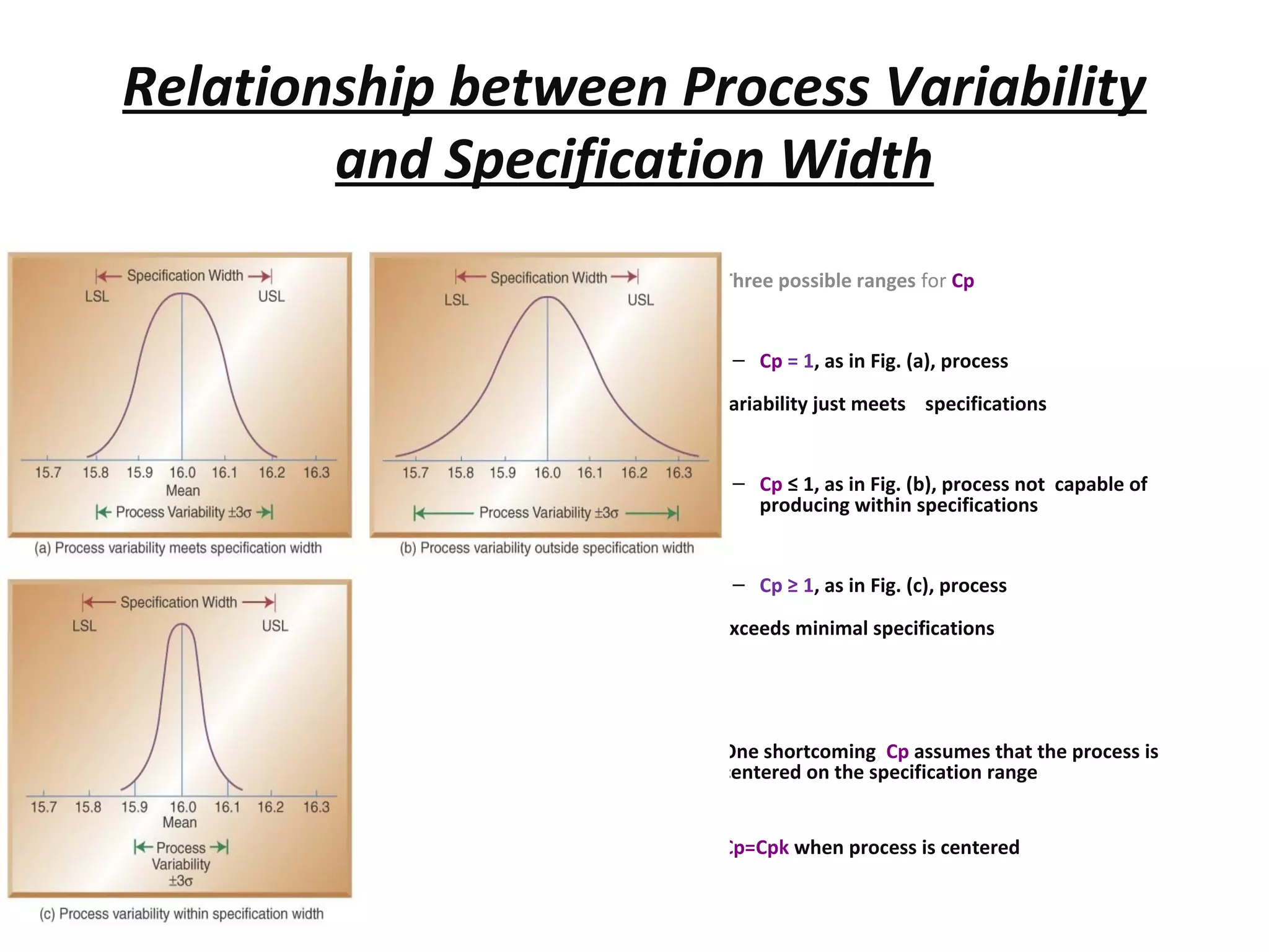
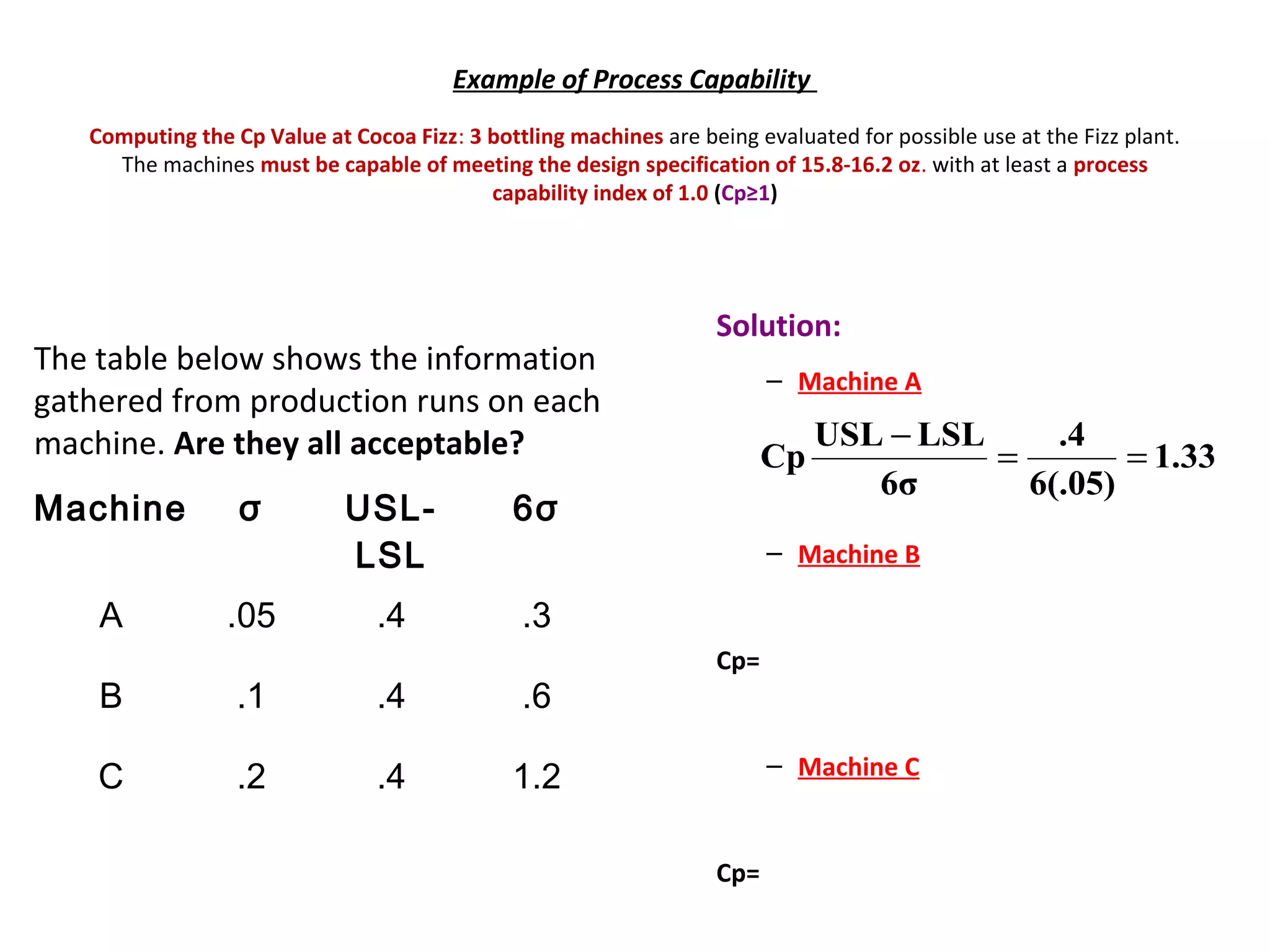
Quality Control and Analysis
Quality is define as customers perception about the degree to which a product or a service meets his expectations.
1.Types of Quality
• Quality of Design
It is concerned with the tightness of specification for manufacturing any product.
• Quality of Performance
It is concerned with how well a product gives its performance. It depends upon quality of design
and quality of conformance.
2. Parameters Governing Quality
• Performance
• Range and type of features
• Reliability and durability
• Maintainability and serviceability
3. Statistical Quality Control (SQC)
It is defined as the quality control system where
statistical techniques are used to control, improve
and maintain quality.
Quantitative aspects of quality management
Statistical quality control Statistical process control
(Acceptance sampling) (Process Control Charts)
Descriptive Statistics
• Descriptive Statistics include:
– The Mean- measure of central
tendency
– The Range- difference between
largest/smallest observations in a
set of data
– Standard Deviation measures the
amount of data dispersion around
mean
– Distribution of Data shape
– Normal or bell shaped or
– Skewed
n
x
x
n
1i
i∑=
=
( )
1n
Xx
σ
n
1i
2
i
−
−
=
∑=
meansampleofmeanstandardσ
deviationstandardProcessσsizesamplen;where
x =
==
Control Charts and Their Types
• The basis of control charts is to checking whether the variation
in the magnitude of a given characteristic of a manufactured
product is arising due to random variation or assignable
variation.
• Random variation: Natural variation or allowable variation,
small magnitude. e.g. length, weight, diameter, time
• Assignable variation: Non-random variation or preventable
variation, relatively high magnitude.
If the variation is arising due to random variation, the process is
said to be under control. But, if the variation is arising due to
assignable variation then the process is said to be out of control.
Types of Control Charts
x
Chart
R
Chart
s
Chart
c
Chart
np
Chart
p
Chart
Variables Attributes
Control Chart
Control Chart for Variable
• The Mean Chart (x-Chart): It shows the centering of the
process and shows the variation in the averages of individual
samples. e.g. length, weight, diameter, time.
• R Chat: It show the variation in the range of the sample.
• Control Unit: For plotting control charts generally ±3σ
selected. Therefore such control charts are known as 3σ
control charts.
• Percentage of values under normal curve
Major Parts of Control Chart
CL
UCL
LC
L
3σ
3σ
Out of control
Out of control
1091 2 3 4 5 6 7 8
Sample Number
QualityScale
Central Line (CL): This indicates the
desired standard or the level of the
process.
Upper Control Limit (UCL): This
indicates the upper limit of tolerance.
Lower Control Limit (LCL): This
indicates the lower limit of tolerance.
If m is the underlying statistic so that
&
CL =
UCL =
LCL =
( ) mE m = µ ( ) 2
Var mm = σ
mµ
3m mµ + σ
3m mµ − σ
Calculation Procedure for x-Bar & R Chart
• Calculate the x-bar and Range for each samples.
• Calculate the grand average ( ) and average range ( ).
Let sample size(n)=5
x R
S. No. 1 2 3 4 5
1
2
. . .
. . .
. . .
N
x R
1X
2X
NX
1R
2R
NR
•For X-Chart
sizesampleson thedependsdanddofvaluethewhere;
RDLCL
RDUCL
N
R......RR
R
43
3
4
N21
R
R
=
=
+++
=
• For R- Chart
N
x
X
N
1i
i∑=
=
x
x
σ
σ
3XLCL
3XUCL
−=
+=
sizesample
deviationstandardProcess
meansampleofmeanstandardwhere;
Here,
=
=
=
=
n
n
x
x
σ
σ
σ
σ
xx
xx
n21
zσxLCL
zσxUCL
sampleeachw/innsobservatioof#theis
(n)andmeanssampleof#theis)(where
n
σ
σ,
...xxx
x x
−=
+=
=
++
=
k
k
Constructing an X-bar Chart:
A quality control inspector at the Cocoa Fizz soft drink company has taken three
samples with four observations each of the volume of bottles filled. If the standard
deviation of the bottling operation is .2 ounces, use the below data to develop
control charts with limits of 3 standard deviations for the 16 oz. bottling operation.
Center line and control limit
formulas
Time 1 Time 2 Time 3
Observation 1 15.8 16.1 16.0
Observation 2 16.0 16.0 15.9
Observation 3 15.8 15.8 15.9
Observation 4 15.9 15.9 15.8
Sample
means (X-
bar)
15.875 15.975 15.9
Sample
ranges (R)
0.2 0.3 0.2
Solution and Control Chart (x-bar)
• Center line (x-double bar):
• Control limits for±3σ limits:
15.92
3
15.915.97515.875
x =
++
=
15.62
4
.2
315.92zσxLCL
16.22
4
.2
315.92zσxUCL
xx
xx
=





−=−=
=





+=+=
Control Chart for Range (R)
• Center Line and Control Limit
formulas:
• Factors for three sigma control
limits
0.00.0(.233)RDLCL
.532.28(.233)RDUCL
.233
3
0.20.30.2
R
3
4
R
R
===
===
=
++
=
Factor for x-Chart
A2 D3 D4
2 1.88 0.00 3.27
3 1.02 0.00 2.57
4 0.73 0.00 2.28
5 0.58 0.00 2.11
6 0.48 0.00 2.00
7 0.42 0.08 1.92
8 0.37 0.14 1.86
9 0.34 0.18 1.82
10 0.31 0.22 1.78
11 0.29 0.26 1.74
12 0.27 0.28 1.72
13 0.25 0.31 1.69
14 0.24 0.33 1.67
15 0.22 0.35 1.65
Factors for R-Chart
Sample Size
(n)
• R- Bar Control Chart
Control Charts for Attributes
P-Charts & C-Charts
• Attributes are discrete events: yes/no or pass/fail
– Use P-Charts for quality characteristics that are discrete and involve
yes/no or good/bad decisions
– Number of leaking caulking tubes in a box of 48
– Number of broken eggs in a carton
– Use C-Charts for discrete defects when there can be more than one
defect per unit
– Number of flaws or stains in a carpet sample cut from a production run
– Number of complaints per customer at a hotel
•P- Chart:
It is also known as fraction defective chart.
This is made for the situation where the sample
size is varying.
Sample No. Size No.(n) No. of
Defectives
Fraction
Defective
1 n1 d1 p1
2 n2 d2 p2
3 n3 d3 p3
: : : :
: : : :
N nn dn pn
InspectedTotal
Defectives#
pCL ==
N
n
)n(sizesampleAverage
N
1i
i∑=
=
( )
( )σzpLCL
σzpUCL
p
p
−=
+=
P-Chart Example:
A production manager for a tire company has inspected the number of defective tires in
five random samples with 20 tires in each sample. The table below shows the number of
defective tires in each sample of 20 tires. Calculate the control limits.
Sample Number
of
Defective
Tires
Number of
Tires in
each
Sample
Proportion
Defective
1 3 20 .15
2 2 20 .10
3 1 20 .05
4 2 20 .10
5 2 20 .05
Total 9 100 .09
Solution:
( )
( ) 0.1023(.064).09σzpLCL
.2823(.064).09σzpUCL
0.64
20
(.09)(.91)
n
)p(1p
σ
.09
100
9
InspectedTotal
Defectives#
pCL
p
p
p
=−=−=−=
=+=+=
==
−
=
====
Control Chart for Defects (C-Chart)
• C-Chart is made of number of defects which are present in a
sample and is made for the situation where the sample size (n) is
constant, n can be equal to 1 or more than one.
• Consider the occurrence of defects in an inspection of product(s).
Suppose that defects occur in this inspection according to Poisson
distribution; that is
Where x is the number of defects and c is known as mean and/or variance of the
Poisson distribution
When the mean number of defects c in the population from which samples are taken
is known
( ) , 0,1, 2, ,
!
c x
e c
P x x
x
−
= = K
ccLCL
ccUCL
samplesof#
complaints#
CL
c
c
z
z
−=
+=
=
Note: If this calculation yields a negative value of
LCL then set LCL=0.
C-Chart Example:
The number of weekly customer complaints are monitored in a
large hotel using a c-chart. Develop three sigma control limits
using the data table below.
Week Number of
Complaints
1 3
2 2
3 3
4 1
5 3
6 3
7 2
8 1
9 3
10 1
Solution:
02.252.232.2ccLCL
6.652.232.2ccUCL
2.2
10
22
samplesof#
complaints#
CL
c
c
=−=−=−=
=+=+=
===
z
z
•np-Chart (Number of Defective chart):
This is known as number of defective chart and is made for the cases
where the sample size (n) is constant.
Sample
number
Sample
size (n)
No. of
defective
(d)
P=d/n
1 n d1 P1=d1/n
2 n d2 P2=d2/n
3 n d3 P3=d3/n
: : : :
: : : :
, n dn Pn=dn/n
N
p
p
N
1i
i∑=
=
pnCL =
)p-(1pn3pnLCL
)p-(1pn3pnUCL
−=
+=
Process Capability
• Product Specifications
– Preset product or service dimensions, tolerances: bottle fill might be 16 oz. ±.2 oz. (15.8oz.-16.2oz.)
– Based on how product is to be used or what the customer expects
• Process Capability – Cp and Cpk
– Assessing capability involves evaluating process variability relative to preset product or service specifications
– Cp assumes that the process is centered in the specification range
– Cpk helps to address a possible lack of centering of the process 6σ
LSLUSL
widthprocess
widthionspecificat
Cp
−
==





 −−
=
3σ
LSLμ
,
3σ
μUSL
minCpk
 Process capability compares the output of in-
control process to the specification limits.
Relationship between Process Variability
and Specification Width
• Three possible ranges for Cp
– Cp = 1, as in Fig. (a), process
variability just meets specifications
– Cp ≤ 1, as in Fig. (b), process not capable of
producing within specifications
– Cp ≥ 1, as in Fig. (c), process
exceeds minimal specifications
• One shortcoming, Cp assumes that the process is
centered on the specification range
• Cp=Cpk when process is centered
Example of Process Capability
Computing the Cp Value at Cocoa Fizz: 3 bottling machines are being evaluated for possible use at the Fizz plant.
The machines must be capable of meeting the design specification of 15.8-16.2 oz. with at least a process
capability index of 1.0 (Cp≥1)
The table below shows the information
gathered from production runs on each
machine. Are they all acceptable?
Solution:
– Machine A
– Machine B
Cp=
– Machine C
Cp=
Machine σ USL-
LSL
6σ
A .05 .4 .3
B .1 .4 .6
C .2 .4 1.2
1.33
6(.05)
.4
6σ
LSLUSL
Cp ==
−
Computing the Cpk Value at Cocoa Fizz
• Design specifications call for a target value of 16.0
±0.2 OZ.
(USL = 16.2 & LSL = 15.8)
• Observed process output has now shifted and has a
µ of 15.9 and a
σ of 0.1 oz.
where: µ= the mean of the process
• Cpk is less than 1, revealing that the process is not
capable.
.33
.3
.1
Cpk
3(.1)
15.815.9
,
3(.1)
15.916.2
minCpk
==





 −−
=

Quality Control Chart

  • 1.
    Quality Control andAnalysis Quality is define as customers perception about the degree to which a product or a service meets his expectations. 1.Types of Quality • Quality of Design It is concerned with the tightness of specification for manufacturing any product. • Quality of Performance It is concerned with how well a product gives its performance. It depends upon quality of design and quality of conformance. 2. Parameters Governing Quality • Performance • Range and type of features • Reliability and durability • Maintainability and serviceability
  • 2.
    3. Statistical QualityControl (SQC) It is defined as the quality control system where statistical techniques are used to control, improve and maintain quality. Quantitative aspects of quality management Statistical quality control Statistical process control (Acceptance sampling) (Process Control Charts)
  • 3.
    Descriptive Statistics • DescriptiveStatistics include: – The Mean- measure of central tendency – The Range- difference between largest/smallest observations in a set of data – Standard Deviation measures the amount of data dispersion around mean – Distribution of Data shape – Normal or bell shaped or – Skewed n x x n 1i i∑= = ( ) 1n Xx σ n 1i 2 i − − = ∑= meansampleofmeanstandardσ deviationstandardProcessσsizesamplen;where x = ==
  • 4.
    Control Charts andTheir Types • The basis of control charts is to checking whether the variation in the magnitude of a given characteristic of a manufactured product is arising due to random variation or assignable variation. • Random variation: Natural variation or allowable variation, small magnitude. e.g. length, weight, diameter, time • Assignable variation: Non-random variation or preventable variation, relatively high magnitude. If the variation is arising due to random variation, the process is said to be under control. But, if the variation is arising due to assignable variation then the process is said to be out of control.
  • 5.
    Types of ControlCharts x Chart R Chart s Chart c Chart np Chart p Chart Variables Attributes Control Chart
  • 6.
    Control Chart forVariable • The Mean Chart (x-Chart): It shows the centering of the process and shows the variation in the averages of individual samples. e.g. length, weight, diameter, time. • R Chat: It show the variation in the range of the sample. • Control Unit: For plotting control charts generally ±3σ selected. Therefore such control charts are known as 3σ control charts. • Percentage of values under normal curve
  • 7.
    Major Parts ofControl Chart CL UCL LC L 3σ 3σ Out of control Out of control 1091 2 3 4 5 6 7 8 Sample Number QualityScale Central Line (CL): This indicates the desired standard or the level of the process. Upper Control Limit (UCL): This indicates the upper limit of tolerance. Lower Control Limit (LCL): This indicates the lower limit of tolerance. If m is the underlying statistic so that & CL = UCL = LCL = ( ) mE m = µ ( ) 2 Var mm = σ mµ 3m mµ + σ 3m mµ − σ
  • 8.
    Calculation Procedure forx-Bar & R Chart • Calculate the x-bar and Range for each samples. • Calculate the grand average ( ) and average range ( ). Let sample size(n)=5 x R S. No. 1 2 3 4 5 1 2 . . . . . . . . . N x R 1X 2X NX 1R 2R NR
  • 9.
    •For X-Chart sizesampleson thedependsdanddofvaluethewhere; RDLCL RDUCL N R......RR R 43 3 4 N21 R R = = +++ = •For R- Chart N x X N 1i i∑= = x x σ σ 3XLCL 3XUCL −= += sizesample deviationstandardProcess meansampleofmeanstandardwhere; Here, = = = = n n x x σ σ σ σ
  • 10.
    xx xx n21 zσxLCL zσxUCL sampleeachw/innsobservatioof#theis (n)andmeanssampleof#theis)(where n σ σ, ...xxx x x −= += = ++ = k k Constructing anX-bar Chart: A quality control inspector at the Cocoa Fizz soft drink company has taken three samples with four observations each of the volume of bottles filled. If the standard deviation of the bottling operation is .2 ounces, use the below data to develop control charts with limits of 3 standard deviations for the 16 oz. bottling operation. Center line and control limit formulas Time 1 Time 2 Time 3 Observation 1 15.8 16.1 16.0 Observation 2 16.0 16.0 15.9 Observation 3 15.8 15.8 15.9 Observation 4 15.9 15.9 15.8 Sample means (X- bar) 15.875 15.975 15.9 Sample ranges (R) 0.2 0.3 0.2
  • 11.
    Solution and ControlChart (x-bar) • Center line (x-double bar): • Control limits for±3σ limits: 15.92 3 15.915.97515.875 x = ++ = 15.62 4 .2 315.92zσxLCL 16.22 4 .2 315.92zσxUCL xx xx =      −=−= =      +=+=
  • 12.
    Control Chart forRange (R) • Center Line and Control Limit formulas: • Factors for three sigma control limits 0.00.0(.233)RDLCL .532.28(.233)RDUCL .233 3 0.20.30.2 R 3 4 R R === === = ++ = Factor for x-Chart A2 D3 D4 2 1.88 0.00 3.27 3 1.02 0.00 2.57 4 0.73 0.00 2.28 5 0.58 0.00 2.11 6 0.48 0.00 2.00 7 0.42 0.08 1.92 8 0.37 0.14 1.86 9 0.34 0.18 1.82 10 0.31 0.22 1.78 11 0.29 0.26 1.74 12 0.27 0.28 1.72 13 0.25 0.31 1.69 14 0.24 0.33 1.67 15 0.22 0.35 1.65 Factors for R-Chart Sample Size (n) • R- Bar Control Chart
  • 13.
    Control Charts forAttributes P-Charts & C-Charts • Attributes are discrete events: yes/no or pass/fail – Use P-Charts for quality characteristics that are discrete and involve yes/no or good/bad decisions – Number of leaking caulking tubes in a box of 48 – Number of broken eggs in a carton – Use C-Charts for discrete defects when there can be more than one defect per unit – Number of flaws or stains in a carpet sample cut from a production run – Number of complaints per customer at a hotel
  • 14.
    •P- Chart: It isalso known as fraction defective chart. This is made for the situation where the sample size is varying. Sample No. Size No.(n) No. of Defectives Fraction Defective 1 n1 d1 p1 2 n2 d2 p2 3 n3 d3 p3 : : : : : : : : N nn dn pn InspectedTotal Defectives# pCL == N n )n(sizesampleAverage N 1i i∑= = ( ) ( )σzpLCL σzpUCL p p −= +=
  • 15.
    P-Chart Example: A productionmanager for a tire company has inspected the number of defective tires in five random samples with 20 tires in each sample. The table below shows the number of defective tires in each sample of 20 tires. Calculate the control limits. Sample Number of Defective Tires Number of Tires in each Sample Proportion Defective 1 3 20 .15 2 2 20 .10 3 1 20 .05 4 2 20 .10 5 2 20 .05 Total 9 100 .09 Solution: ( ) ( ) 0.1023(.064).09σzpLCL .2823(.064).09σzpUCL 0.64 20 (.09)(.91) n )p(1p σ .09 100 9 InspectedTotal Defectives# pCL p p p =−=−=−= =+=+= == − = ====
  • 16.
    Control Chart forDefects (C-Chart) • C-Chart is made of number of defects which are present in a sample and is made for the situation where the sample size (n) is constant, n can be equal to 1 or more than one. • Consider the occurrence of defects in an inspection of product(s). Suppose that defects occur in this inspection according to Poisson distribution; that is Where x is the number of defects and c is known as mean and/or variance of the Poisson distribution When the mean number of defects c in the population from which samples are taken is known ( ) , 0,1, 2, , ! c x e c P x x x − = = K ccLCL ccUCL samplesof# complaints# CL c c z z −= += = Note: If this calculation yields a negative value of LCL then set LCL=0.
  • 17.
    C-Chart Example: The numberof weekly customer complaints are monitored in a large hotel using a c-chart. Develop three sigma control limits using the data table below. Week Number of Complaints 1 3 2 2 3 3 4 1 5 3 6 3 7 2 8 1 9 3 10 1 Solution: 02.252.232.2ccLCL 6.652.232.2ccUCL 2.2 10 22 samplesof# complaints# CL c c =−=−=−= =+=+= === z z
  • 18.
    •np-Chart (Number ofDefective chart): This is known as number of defective chart and is made for the cases where the sample size (n) is constant. Sample number Sample size (n) No. of defective (d) P=d/n 1 n d1 P1=d1/n 2 n d2 P2=d2/n 3 n d3 P3=d3/n : : : : : : : : , n dn Pn=dn/n N p p N 1i i∑= = pnCL = )p-(1pn3pnLCL )p-(1pn3pnUCL −= +=
  • 19.
    Process Capability • ProductSpecifications – Preset product or service dimensions, tolerances: bottle fill might be 16 oz. ±.2 oz. (15.8oz.-16.2oz.) – Based on how product is to be used or what the customer expects • Process Capability – Cp and Cpk – Assessing capability involves evaluating process variability relative to preset product or service specifications – Cp assumes that the process is centered in the specification range – Cpk helps to address a possible lack of centering of the process 6σ LSLUSL widthprocess widthionspecificat Cp − ==       −− = 3σ LSLμ , 3σ μUSL minCpk  Process capability compares the output of in- control process to the specification limits.
  • 20.
    Relationship between ProcessVariability and Specification Width • Three possible ranges for Cp – Cp = 1, as in Fig. (a), process variability just meets specifications – Cp ≤ 1, as in Fig. (b), process not capable of producing within specifications – Cp ≥ 1, as in Fig. (c), process exceeds minimal specifications • One shortcoming, Cp assumes that the process is centered on the specification range • Cp=Cpk when process is centered
  • 21.
    Example of ProcessCapability Computing the Cp Value at Cocoa Fizz: 3 bottling machines are being evaluated for possible use at the Fizz plant. The machines must be capable of meeting the design specification of 15.8-16.2 oz. with at least a process capability index of 1.0 (Cp≥1) The table below shows the information gathered from production runs on each machine. Are they all acceptable? Solution: – Machine A – Machine B Cp= – Machine C Cp= Machine σ USL- LSL 6σ A .05 .4 .3 B .1 .4 .6 C .2 .4 1.2 1.33 6(.05) .4 6σ LSLUSL Cp == −
  • 22.
    Computing the CpkValue at Cocoa Fizz • Design specifications call for a target value of 16.0 ±0.2 OZ. (USL = 16.2 & LSL = 15.8) • Observed process output has now shifted and has a µ of 15.9 and a σ of 0.1 oz. where: µ= the mean of the process • Cpk is less than 1, revealing that the process is not capable. .33 .3 .1 Cpk 3(.1) 15.815.9 , 3(.1) 15.916.2 minCpk ==       −− =

Editor's Notes

  • #3 SPC minimizes the defective items produced thus it is a preventive measur. <number>
  • #8 <number>