![2013/05/22
3
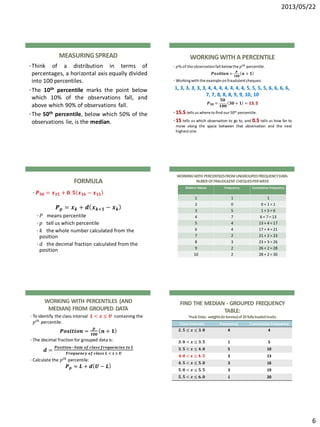
GRAPH: The MODE = 4
0
1
2
3
4
5
6
7
8
1 2 3 4 5 6 7 8 9 10
Frequency
Frequency
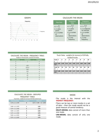
Call Centre Data: waiting times (in seconds)
for 35 randomly selected customers
C1 2 3 4 5 6 7 8 9 10 11 12
75 37 13 90 45 23 104 135 30 73 34 12
C13 14 15 16 17 18 19 20 21 22 23 24
38 40 22 47 26 57 65 33 9 85 87 16
C25 26 27 28 29 30 31 32 33 34 35
102 115 68 29 142 5 15 10 25 41 49
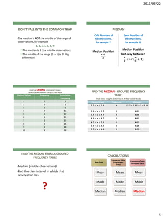
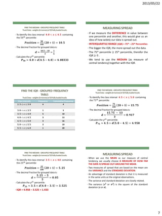
FREQUENCY TABLE: The MODAL CLASS is the
interval 𝟐𝟓 < 𝒙 ≤ 𝟓𝟎
Class Intervals TallyMarks Frequency
0 ≤ 𝑥 ≤ 25 //// //// 10
25 < 𝑥 ≤ 50 //// //// / 11
50 < 𝑥 ≤ 75 //// / 6
75 < 𝑥 ≤ 100 /// 3
100 < 𝑥 ≤ 125 /// 3
125 < 𝑥 ≤ 150 // 2
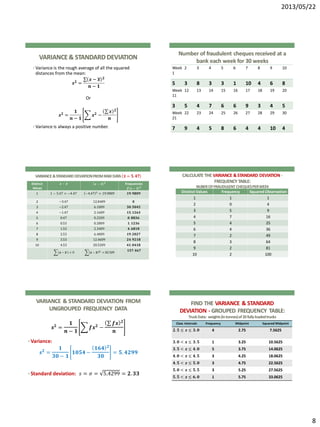
HISTOGRAM: MODAL CLASS (𝟐𝟓 < 𝒙 ≤ 𝟓𝟎]
0
2
4
6
8
10
12
Intervals
[0;25]
(25;50]
(50;75]
(75;100]
(100;125]
(125;150]
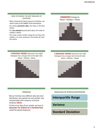
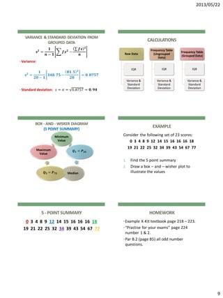
THE MEDIAN – RAW DATA:
Numberoffraudulentchequesreceived atabankeach weekfor30weeks
Week
1
2 3 4 5 6 7 8 9 10
5 3 8 3 3 1 10 4 6 8
Week
11
12 13 14 15 16 17 18 19 20
3 5 4 7 6 6 9 3 4 5
Week
21
22 23 24 25 26 27 28 29 30
7 9 4 5 8 6 4 4 10 4
MEDIAN
• Median = 5
• Put all observations in order from smallest to
largest, then the middle observation is the
MEDIAN.
1, 3, 3, 3, 3, 3, 4, 4, 4, 4, 4, 4, 4, 5, 5, 5,
5, 6, 6, 6, 6, 7, 7, 8, 8, 8, 9, 9, 10, 10](https://image.slidesharecdn.com/chapter9learningmoreaboutsampledata1-130607064111-phpapp02/85/Chapter-9-learning-more-about-sample-data-1-3-320.jpg)

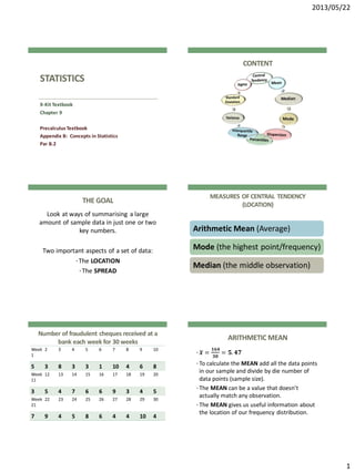
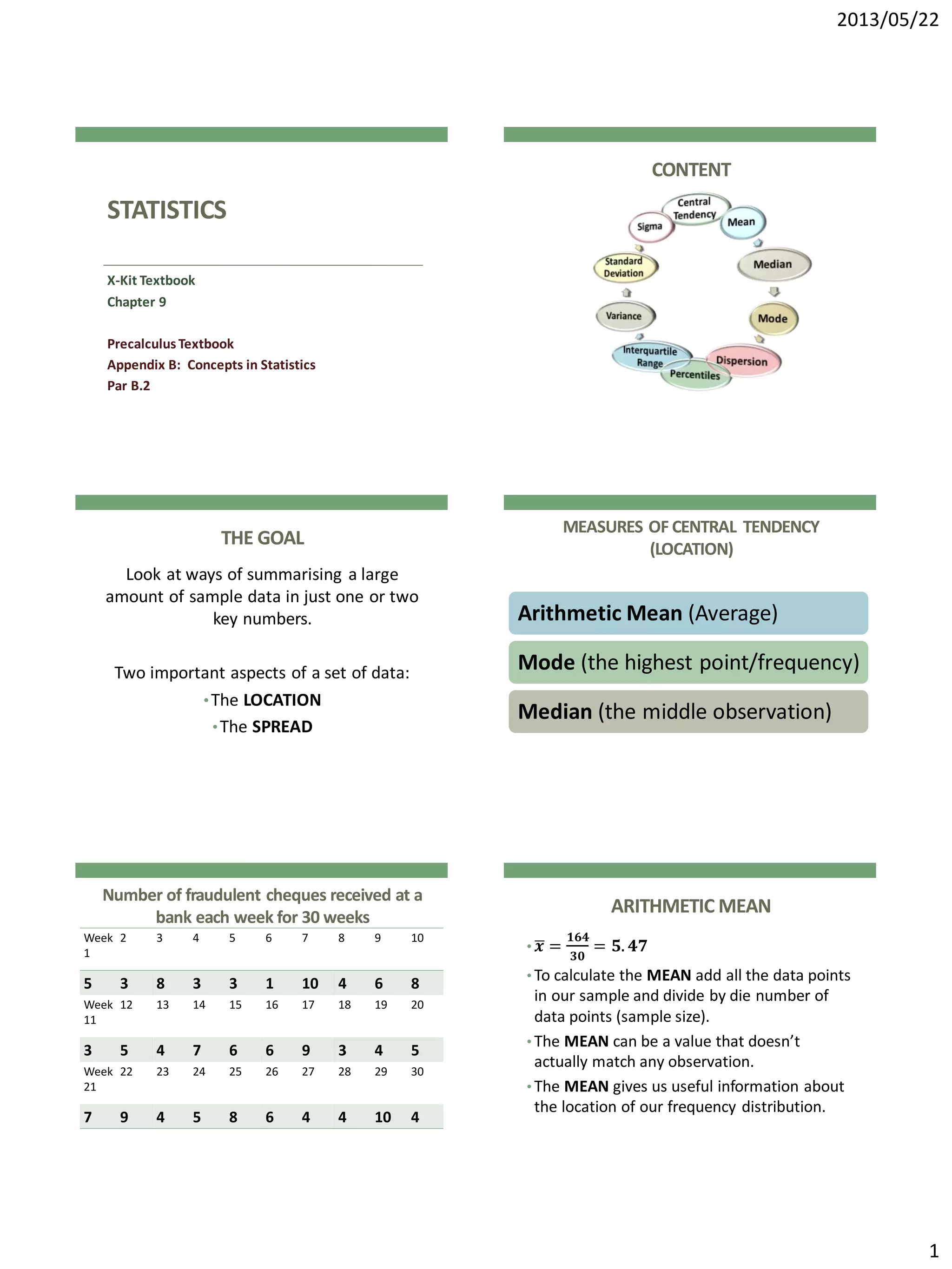
The document discusses various measures of central tendency and spread that can be used to summarize sample data. It describes the arithmetic mean as the average value found by summing all data points and dividing by the sample size. The mode is defined as the most frequent data point. The median is the middle value when data is arranged in order. The interquartile range is introduced as a measure of spread or dispersion in the data. Formulas are provided for calculating these metrics from both raw and grouped frequency data.