Download to read offline


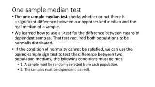
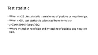
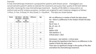
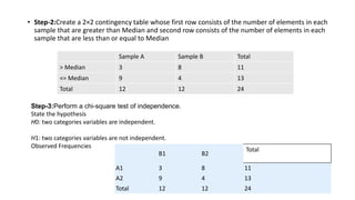
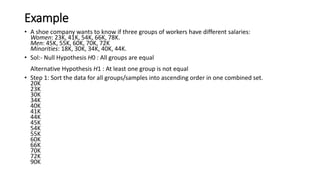
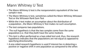
![• Perform Kruskal wallis test for the following data:-
8,5,7,11,9,6 – 25.5
10,12,11,9,13,12 - 64
11,14,10,16,17,12 – 87.5
18,20,16,15,14,22 - 123
• Significance Level α=0.05 and One-tailed test.
• 12/24*25[(25.52 + 642 + 87.52 + 1232 )/6] -3(24+1)
• H= 16.825
• Critical value = 7.815](https://image.slidesharecdn.com/non-parametric-tests-mod-3-210530083105/85/Non-parametric-tests-30-320.jpg)

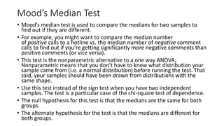
The document discusses several non-parametric tests that can be used as alternatives to parametric tests when the assumptions of parametric tests are violated. Specifically, it discusses: 1. The sign test and one sample median test, which can be used instead of t-tests when the data is skewed or not normally distributed. 2. Mood's median test, which compares the medians of two independent samples and is the nonparametric version of a one-way ANOVA. 3. The Kruskal-Wallis test, which determines if there are differences in medians across three or more groups and is the nonparametric version of a one-way ANOVA.


![제 23회 보아즈(BOAZ) 빅데이터 컨퍼런스 - [MBOAX] : ABSA를 활용한 소비자 반응 분석 기반 운영 효율화 대시보드 설계](https://cdn.slidesharecdn.com/ss_thumbnails/3-1boaz23rdconferencemboax-260203102709-9d519923-thumbnail.jpg?width=640&height=640&fit=bounds)


