CONVERGENCE ANALYSIS OF NEWTON-COTES METHODS: OPTIMIZING SUB-INTERVALS SELECTION FOR PRECISE INTEGRAL APPROXIMATION

Applied Mathematics and Sciences: An International Journal (MathSJ) Vol.11, No.1/2, June 2024
DOI : 10.5121/mathsj.2024.11201 1
CONVERGENCE ANALYSIS OF NEWTON-COTES
METHODS: OPTIMIZING SUB-INTERVALS
SELECTION FOR PRECISE
INTEGRAL APPROXIMATION
Lea A. Catapang1
, James Ray Mendaje1
and Venus D. Siong2
1
School of Foundation, Bahrain Polytechnic, Bahrain
2
College of Arts and Sciences, Don Mariano Marcos State University, Philippines
ABSTRACT
This study explored the piecewise approach of the closed Newton-Cotes quadrature formulas (Trapezoidal,
Simpson’s 1/3, and 3/8 rules) and how well they work with different kinds of functions in terms of
convergence and accuracy. MATHEMATICA software was used to approximate the integrals and
determine their errors, allowing for a comparison of convergence and accuracy. Simpson’s 1/3 and 3/8
rules consistently outperformed the trapezoidal rule, demonstrating faster convergence and greater
accuracy across a wide range of functions. However, as tolerance levels increased to a considerable
magnitude, Simpson’s 3/8 rule emerged as the most robust among the three methods. We recommend
investigating various domains to substantiate the findings of this study including a comprehensive error
analysis that includes truncation error, round-off error, and error bounds to provide a more detailed
understanding of the sources and magnitude of errors and to include higher-dimensional integrals to
provide valuable insights into the robustness of these methods.
KEYWORDS
Numerical Quadrature, Newton-Cotes, Trapezoidal Rule, Simpson’s 1/3 rule, Simpson’s 3/8 rule
1. INTRODUCTION
The Newton-Cotes quadrature methods are a class of numerical integration techniques based on
polynomial interpolation over a set of equally spaced nodes [1]. These techniques provide a direct
approximation of definite integral . However, they can quickly become unstable
when applied to functions with distinct characteristics specially those that are not well-
approximated by low-degree polynomials over large intervals. This leads to a substantial increase
of error, as the polynomial interpolant may not accurately capture the behaviour of the integrand
over a large interval.
The Newton-Cotes formulas are obtained by interpolating polynomials which approximate the
tabulated function . Then integrating the function over some interval divided
into equal sub-intervals such that and [2]. The two types of Newton-
Cotes quadrature methods are open and closed. The -point closed Newton-Cotes method
includes endpoints of the closed interval as nodes. It uses nodes
[3]. Unlike
closed Newton-Cotes, open Newton-Cotes formulas do not include the endpoints of .

2
The most recognized closed Newton-Cotes formulas are the trapezoidal rule and Simpson’s 1/3
and 3/8 rules, mainly because of their balance of simplicity and preciseness. These methods are
widely applied across various areas of study, such as engineering, economics and finance,
computational science, and more [4]. Trapezoidal rule and Simpson’s rule are interpolatory
quadrature based on linear and quadratic interpolants, respectively [5]. These low-order rules are
often slow to converge and return inaccurate results over large intervals due to the oscillatory
nature of high-degree polynomials.
High-order quadrature techniques would be necessary to integrate high-degree polynomials,
however the values of the coefficients in these techniques are difficult to obtain and often
numerically unstable [1][3]. Alternatively, the Composite Quadrature rules for trapezoidal and
Simpson’s are simpler approach and considered an effective way to increase the accuracy of the
result when integrating high-degree polynomials. These rules involve partitioning the interval
into subintervals then using low-order interpolants (e.g. Trapezoidal and Simpson) to
approximate the integrals in each subinterval.
The composite approach in numerical quadrature, particularly, using low-order Newton-Cotes
methods like the trapezoidal rule and Simpson's rule has been extensively studied due to its
practical advantages in improving accuracy and managing the convergence of integral
approximations. The study by Udin, M.J.et al evaluated and compared the performance of
Trapezoidal, Simpson’s 1/3, and 3/8 rules in terms of accuracy and efficiency, utilizing error
analysis to determine which method performs better in providing accurate results [6]. Daan
Huybrechs, reviewed and presented the difference between the low-order variants of the class of
Newton-Cotes quadrature and the high-order quadrature (Least-Square quadrature) in terms of
numerical stability and convergence properties [1]. Yalda Qani used the advanced family of
closed Newton–Cotes numerical composite formulas to demonstrate some of the computational
capabilities of the Maple package [7]. In the A.H. Nzokem study, he implemented both analytical
and numerical methods (composite Newton-Cotes quadrature formulas) in solving the Gamma
Distribution Hazard function [8]. Sheehan Olver investigated and explored the numerical
integration of highly oscillatory functions, over both univariate and multivariate domains, using
the combination of Filon-type methods and Levin-type methods [9]. Furthermore, Hamid
Mottaghi Golshan proposed a numerical iterative method based on Picard iterations and Newton-
Cotes rules that can be used to approximate the multidimensional Fredholm–Urysohn integral
equation of the second kind [10]. The study of Magalhaes, P. et al. discussed and compared the
closed and open Newton-Cotes quadrature formula, utilizing twenty segments to assess the
accuracy and convergence of the two methods [11]. In the work of Ali, A. J. et al, they utilized
error and stability analysis to evaluate the degree of accuracy of analytical, numerical
(Trapezoidal and Simpson’s 1/3 and 3/8 rules), and software-assisted (MatLab) methods [12].
Likewise, Erme Sermutlu conducted a study utilizing MatLab and error analysis to compare
Newton-Cotes and Gauss quadrature methods over the same number of intervals for diverse types
of functions [13]. Additionally, John Roumeliotis used the software-assisted method (Maple) to
prove the Ostrowski and corrected Trapezoidal inequalities and stated two new fourth-order
quadrature formula [14]. Wu, J et. Al. explored and used the composite Newton-Cotes methods
for computation of Hadamard finite-part integral with the second order singularity focusing on
their pointwise superconvergence properties [15]. And, in the study conducted by Clarence Burg,
he presented a new closed Newton–Cotes type of quadrature formula that uses first and higher
order derivatives to increase the order of accuracy of the numerical approximations of definite
integrals [16].
This paper, like the cited studies, aims to investigate the Newton-Cotes quadrature methods
(Trapezoidal and Simpson’s rules) for approximating definite integrals and analyse their
convergence and accuracy. However, it will focus on the piecewise approach (composite rules) of

3
the closed Newton-Cotes quadrature methods and explore their applicability to various special
function types. It will also determine how the selection of sub-intervals affects the accuracy and
convergence of these approaches.
2. MATERIALS AND METHODS
Presented in this section is the piecewise approach of the three commonly used closed Newton-
Cotes quadrature formulas.
2.1. Closed Newton-Cotes Quadrature Formulas
Newton–Cotes methods consist of approximating the integrand by a polynomial of degree ,
which matches at evenly spaced nodes [10]. The -point closed Newton-Cotes
method includes endpoints of the closed interval as nodes [3, p.198]. It uses nodes
assuming the
form
(2.1)
where the weight
(2.2)
Using the first order Lagrange interpolating polynomial, (2.1) and (2.2) return
with,
and
Combining and simplifying, we obtain the standard trapezoidal rule,
(2.3)
Since (2.3) can also be expressed as
In a similar manner, using the second-order Lagrange interpolating polynomials, (2.1) and (2.2)
give
with,

4
We obtain the standard 1/3 Simpson’s rule, which is one of the most recognized closed Newton-
Cotes quadrature approaches in practice.
(2.4)
Since (2.4) can also be written as
Likewise, utilizing the third-order Lagrange interpolating polynomial (2.1) becomes,
with

5
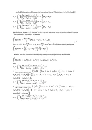
Combining and simplifying, we obtain the 3/8 Simpson’s rule
(2.5)
Since (2.5) can be
expressed as
2.2. Measure of Exactness
Definition 2.1 [5, p. 121] An interpolatory quadrature rule has degree of exactness (degree of
precision) if for all (polynomial interpolant),
The definition indicates that a degree- quadrature method has a degree of exactness
This further implies that it can exactly integrate . However, there are exceptional cases
wherein a degree- interpolant can also exactly integrate higher degree polynomials.
Consequently, the degree of precision of trapezoidal rule and Simpson’s rules are one and three,
respectively.

6
2.3. Error Analysis for Closed Newton-Cotes Quadrature Methods
The following theorem serves as basis for error analysis of the closed Newton-Cotes quadrature
formulas since they are founded on polynomial interpolation and weighted sum of function
values at specific nodes.
Theorem 2.1 [5, p. 217] (Interpolation Error Formula) Suppose and let
denote the polynomial that interpolates { for distinct points
Then for every there exist such that
(2.6)
From this formula follows a bound for the worst error over :
Proof. Let be some arbitrary points in the interval and let be
the interpolation error of . We want an expression to describe If for any
then and choosing arbitrary in returns (2.6).
Now, suppose for all , to describe we define a function for in
[ by
Since and , it follows that For , we obtain
Furthermore,
Hence, and at the distinct numbers By Rolle’s
theorem there exist a number in for which . And the derivative of
is
Since is of degree at most , then the derivative . Additionally,
is of degree polynomial, thus

7
Equation (2.6.1) becomes,
Therefore, for some
Theorem 2.2 [3, p. 198] Suppose that denotes The -point closed
Newton-Cotes formula with . There exist for which
(2.7)
If is even and and
(2.8)
If is odd and
Using this theorem with (2.8) returns
From (2.3) with , we obtain the standard trapezoidal rule
with its error term,
(2.9)
where .
Similarly, we obtain the standard Simpson’s 1/3 rule with its error term using (2.4) with
and (2.7) becomes,

8
(2.10)
where .
Simpson’s 3/8 rule with its error term is obtained using (2.5) with
and (2.8) yields,
(2.11)
where
These indicates that the degree of precision of (2.7) is and (2.8) is although the
interpolation polynomial is of degree at most .
2.4. Composite Rules
Composite quadrature rules for trapezoidal and Simpson’s are simpler approach and is considered
an effective way to increase the accuracy of the result when integrating high-degree polynomials.
These rules involve partitioning the interval into subintervals then using the low-order
interpolants such as the standard Newton-Cotes methods on each subinterval.
2.4.1. Composite Trapezoidal Rule
Suppose interval is partitioned into intervals [ by
. Employing the standard trapezoidal rule on subinterval
returns
(2.12)
Since application of standard Newton-Cotes methods consider that is evaluated at equally
spaced nodes between and , then (2.12)
returns the composite trapezoidal rule,
(2.13)

9
Theorem2.3 [3, p. 206]Let , and .
There exists for which the Composite Trapezoidal rule for subintervals can be
written with its error term as
(2.14)
The error term in (2.14) can be derived from the summation of all errors in the application of
standard trapezoidal rule on each subinterval. Thus,
for .
Since then by Extreme Value Theorem,
we have, n
and,
By Intermediate Value Theorem, there is such that
Hence,
and since , then
It is intriguing to note that the error term for the composite trapezoidal rule is not
that we have in (2.9). These are not comparable because for standard trapezoidal rule is fixed at
since , but for composite trapezoidal rule for positive integer .
2.4.2. Composite Simpson’s Rule
Composite Simpson’s 1/3 rule is obtained in an equivalent manner (as Composite Trapezoidal
rule); however, we choose an even integer , partitioning the interval into subintervals,
then applying the standard Simpson’s rule on each consecutive pair of subintervals. Applying
some algebraic manipulations, we obtain

10
(2.15)
Theorem 2.4 [3, p. 206] Let be even , and
. There exists for which the composite Simpson’s
rule for subintervals can be written with its error term as
(2.16)
Similarly, the error term in (2.16) can be derived from the summation of all errors in the
application of standard Simpson’s rule on each consecutive pair of subintervals. Thus,
for for .
Since then by Extreme Value Theorem,
we have,
and
By Intermediate Value Theorem, there is such that,
Hence
and since , then

11
We can also observe that the error term for the Composite Simpson’s rule is , instead of
which was the error in the standard Simpson’s rule (2.10). This is simply because the in
standard Simpson’s rule is fixed at rule while in composite Simpson’s rule it is rule
for an even integer
2.5. Mathematica Software
MATHEMATICA is considered a definitive system for modern technical computing [18]. It is
widely used in highly computational environments (both numerical and symbolic) because of its
robust and comprehensive features, which allow flexibility and reliability. We use
MATHEMATICA not only to ensure accuracy and precision of the results but also to visualize
and observe the behaviours of the functions in the three methods employed.
3. RESULTS AND DISCUSSION
This study investigates the robustness and accuracy of composite trapezoidal rule, Simpson’s 1/3
rule, and Simpson’s 3/8 rule to approximate the definite integrals of the standard normal
probability density function, incomplete gamma function, the Fresnel sine function, and
Dawson’s integral These functions hold significant importance and find extensive applications in
various disciplines such as Statistics, Business, and Engineering. The outcomes are discussed in
this section.
3.1. Standard Normal Probability Density Function
The standard normal probability density function is given by . The function is
the basis of calculating the area under the normal curve by determining the definite integral given
a particular interval. However, due to the complexity of the function, it is tedious to determine the
integral. For this reason, numerical integration is used to estimate the value within a given
domain.
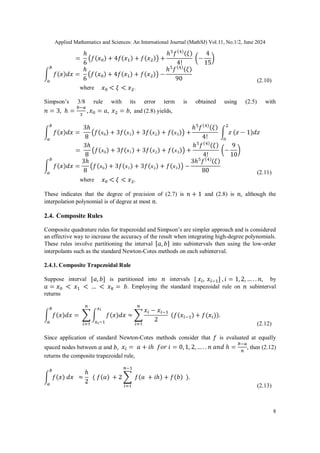
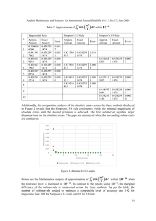
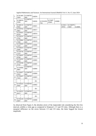
Table 1 displays the results of approximating standard normal probability density function from 0
to 1. This is particularly the area of the normal curve from to
The table shows that both Simpson’s 1/3 rule and 3/8 rules are the most efficient in terms
approximating the integral since it only takes 2 subintervals, and for the 1/3 rule
and and for the 3/8 rule for the approximate value to converge with actual value
considering the absolute errors within tolerance level. The trapezoidal rule on the other
hand requires a significantly larger number of subintervals to achieve a comparable level of
accuracy, requiring 21 subintervals to approach the exact value.

12
Table 1. Approximation of within
n
Trapezoidal Rule Simpson's 1/3 Rule Simpson's 3/8 Rule
Approx.
Answer
Exact
Answer
Abs.
Error
Approx.
Answer
Exact
Answer
Abs.
Error
Approx.
Answer
Exact
Answer
Abs.
Error
1
0.3204565
025
0.3413447
461 0.0209
2
0.3362609
146
0.3413447
461 0.0051
0.3415290
520
0.3413447
461 0.0002
3
0.3390959
119
0.3413447
461 0.0022
0.3414258
380
0.3413447
461
0.000
1
4
0.3400818
445
0.3413447
461 0.0013
0.3413554
879
0.3413447
461 0.0000
5
0.3405370
985
0.3413447
461 0.0008
6
0.3407841
090
0.3413447
461 0.0006
0.3413495
080
0.3413447
461
0.000
0
7
0.3409329
509
0.3413447
461 0.0004
8
0.3410295
157
0.3413447
461 0.0003
9
0.3410957
025
0.3413447
461 0.0002
10
0.3411430
365
0.3413447
461 0.0002
11
0.3411780
536
0.3413447
461 0.0002
12
0.3412046
843
0.3413447
461 0.0001
:
:
:
:
:
:
-do-
21
0.3412990
187
0.3413447
461 0.0000
Although both Simpson’s 1/3 and 3/8 rules require the same number of subintervals to achieve
convergence, a closer examination reveals that the Simpson’s 3/8 rule yields a smaller absolute
error before reaching convergence with the true value. It can be noted in Figure. 1 that there is a
significant difference of the absolute error of the trapezoidal Rule compared to the other methods.
A large gap of the errors is observed on the initial subintervals until the desired tolerance level is
attained. On the other hand, there is a marginal difference between the errors of 1/3 rule and 3/8
rule.

13
Figure 1. Absolute Error Graphs
Below are the Mathematica outputs of approximation of within :
Absolute error set to be below:1.*10^-10
Searching for n that satisfies absolute error less than:1.*10^-10
**********************TRAPEZOIDAL RULE****************************
TOL met at n=9000, Absolute error at:2.489414785*10^-10
n=9000 approx: 0.3413447458 exact: 0.3413447461 Abs error : 2.489414785*10^-10
**********************SIMPSONS 1/3 RULE****************************
**********************SIMPSONS 3/8 RULE****************************
n=90, approx: 0.3413447458 exact: 0.3413447461 Abs error : 9.220813002*10^-11
As revealed by the outputs, if we increase the tolerance level for absolute error to be within
, there is a significance increase of the values of the subintervals across the three methods
for the approximate value to converge with the exact value. Specifically, it necessitates 9000
subintervals for the trapezoidal rule and 37 and 30 for 1/3 and 3/8 Simpsons rules, respectively.
In the field of numerical integration, higher tolerance level indicates better precision and
accuracy.
3.2. Fresnel Sine Function
The Fresnel sine integral, is widely used in the field of optics and used
in the calculation of electromagnetic field density. The approximation of the function at is
scrutinized in this study. The results in Table 2 indicates that there is a lesser variation in terms of
the convergence behaviour across the 3 methods in approximating the definite integral
considering the tolerance level of . It can be observed from the results that it only requires
fewer subintervals of the intervals to achieve an approximation that closely aligns with the true
value. The trapezoidal rule necessitated the use of 6 subintervals to produce an approximate value
that converged with the exact value. In contrast, both Simpson’s 1/3 and 3/8 rules only required 4
to reach a similar level of accuracy.

14
n
Approx.
Answer
Exact
Answer
Error
Approx.
Answer
Exact
Answer
Error
Approx.
Answer
Exact
Answer
Error
1
0.500000
0000
0.438259
1474
0.061
7
2
0.441341
7162
0.438259
1474
0.003
1
0.421788
955
0.438259
1474
0.016
5
3
0.438811
9291
0.438259
1474
0.000
6
0.431163
4203
0.438259
1474
0.007
1
4
0.438427
7565
0.438259
1474
0.000
2
0.437456
437
0.438259
1474
0.000
8
5
0.438327
0254
0.438259
1474
0.000
1
6
0.438291
5734
0.438259
1474
0.000
0
0.438118
121
0.438259
1474
0.000
1
0.437910
3055
0.438259
1474
0.000
3
8
0.438216
495
0.438259
1474
0.000
0
9
0.438197
1694
0.438259
1474
0.000
1
12
0.438240
3145
0.438259
1474
0.000
0
Additionally, the comparative analysis of the absolute errors across the three methods displayed
in Figure 2 reveals that the Simpson's 3/8 rule consistently yields the minimal magnitudes of
absolute errors until the desired precision is achieved. The first subinterval signifies larger
disproportions on the absolute errors. The gaps are minimized when the succeeding subintervals
are considered.
Below are the Mathematica outputs of approximation of within when
the tolerance level is increased to . In contrast to the results using the marginal
difference of the subintervals is maintained across the three methods. As per the table, the
number of subintervals needed to maintain a comparable level of accuracy are: 142 for
trapezoidal rule, 101 for Simpson’s 1/3 rule, and 83 for 3/8 rule.

15
**********************SIMPSONS 1/3 RULE****************************
**********************SIMPSONS 3/8 RULE****************************
3.3. Incomplete Gamma Function
The incomplete gamma function given by is commonly applied in the
field of heat conduction, probability theory, and Fourier and Laplace transformations. The
convergence analysis to approximate the value of the incomplete gamma function utilizing
on the interval within is presented in Table 3.
n
Approx.
Answer
Exact
Answer
Error
Approx.
Answer
Exact
Answer
Error
Approx.
Answer
Exact
Answer
Error
1
0.18393
97206
0.264241
1177
0.080
3
2
0.24360
25252
0.264241
1177
0.020
6
0.263490
1268
0.264241
1177
0.000
8
3
0.25502
05234
0.264241
1177
0.009
2
0.263905
6237
0.264241
1177
0.000
3
4
0.25904
50402
0.264241
1177
0.005
2
0.264192
5452
0.264241
1177
0.000
0
5
0.26091
28085
0.264241
1177
0.003
3
6
0.26192
87269
0.264241
1177
0.002
3
0.264219
5021
0.264241
1177
0.000
0
7
0.26254
17462
0.264241
1177
0.001
7
8
0.26293
98017
0.264241
1177
0.001
3
9
0.26321
27902
0.264241
1177
0.001
0
10
0.26340
80987
0.264241
1177
0.000
8
n
Trapezoidal Rule
Approx.
Answer
Exact
Answer
Error
11
0.26355
26272
0.264241
1177
0.000
7
12
0.26366
25656
0.264241
1177
0.000
6

16
13
0.26374
81311
0.264241
1177
0.000
5
14
0.26381
60294
0.264241
1177
0.000
4
15
0.26387
08094
0.264241
1177
0.000
4
16
0.26391
56448
0.264241
1177
0.000
3
17
0.26395
28047
0.264241
1177
0.000
3
18
0.26398
39460
0.264241
1177
0.000
3
19
0.26401
03015
0.264241
1177
0.000
2
:
:
:
:
:
:
-do-
24
0.26409
64512
0.264241
1177
0.000
1
:
:
:
:
:
:
-do-
41
0.26419
15451
0.264241
1177
0.000
0
There is an exceptionally large discrepancy in terms of the robustness of the trapezoidal rule as
compared to Simpson’s 1/8 and 3/8 rules. To arrive at the desired accuracy level, the trapezoidal
rule required more than 20 times the number of subintervals of the Simpsons rules, and
subintervals for the 1/3 rule and and for the 3/8 rule.
Relative to the results of the other two functions, the 3/8 rule maintained the lowest absolute error
as the value converges the exact answer as displayed in Figure 3. It can be noted from the graph
that in the first few values of subintervals, the absolute errors of utilizing the trapezoidal method
are significantly larger in contrast to the other 2 methods. Simpson’s 1/3 and 3/8 rules exhibits no
significant difference in the errors.

17
Mathematica outputs of approximation of within below compares the
trapezoidal rule, Simpson's 1/3 rule, and Simpson's 3/8 rule highlighting the number of
subintervals needed to achieve an absolute error when the tolerance level is within The
trapezoidal rule required 9000 subintervals to converge with the true value indicating slow
convergence. This is a significant increase when compared to the tolerance level.
Simpson's 1/3 rule achieved the target accuracy with 52 subintervals while the Simpson's 3/8 rule
met the tolerance with 44 subintervals.
**********************SIMPSONS 1/3 RULE****************************
**********************SIMPSONS 3/8 RULE****************************
3.4. Dawson’s Integral
The Dawson’s integral, , bears important contribution in the concept of
heat conduction and the theory of electrical oscillations of special vacuum tubes. Table 4 shows
the results when approximating the value of the Dawson’s integral on the interval
Comparative analysis with the results obtained in incomplete gamma function shows the same
convergence behaviour using the trapezoidal rule. The data further reveals that it takes 58
subintervals to attain the targeted level of precision. The magnitude is significantly larger as
compared to the outcomes of Simpson’s 1/3 and 3/8 rules. It is apparent on the results that the 3/8
rule is the most efficient method, requiring only 3 subintervals ( , 6, and 9), in comparison
to the 1/3 rule, which demands 4 subintervals ( , 4, 6, and 8) for the approximate answer to
converge with the exact answer.
n
Approx.
Answer
Exact
Answer
Error
Approx.
Answer
Exact
Answer
Error
Approx.
Answer
Exact
Answer
Error
1
0.683939
7206
0.5380795
069
0.1459
2
0.578153
1367
0.5380795
069
0.0401
0.5428909
420
0.53807
95069
0.0048
3
0.556268
4773
0.5380795
069
0.0182
0.54030
95719
0.538079
5069 0.0022
4
0.548390
1066
0.5380795
069
0.0103
0.5384690
966
0.53807
95069
0.0004
5
0.544702
3760
0.5380795
069
0.0066
6
0.542687
9211
0.5380795
069
0.0046
0.5381610
690
0.53807
95069
0.0001
0.53825
47691
0.538079
5069 0.0002

18
7
0.541469
3850
0.5380795
069
0.0034
8
0.540676
9309
0.5380795
069 0.0026 0.5381058
724
0.53807
95069
0.0000
9
0.540132
9056
0.5380795
069
0.0021
0.53811
59591
0.538079
5069 0.0000
10
0.539743
4061
0.5380795
069
0.0017
11
0.539455
0259
0.5380795
069
0.0014
12
0.539235
5782
0.5380795
069
0.0012
13
0.539064
7298
0.5380795
069
0.0010
14
0.538929
1253
0.5380795
069
0.0008
15
0.538819
6999
0.5380795
069
0.0007
16
0.538730
1253
0.5380795
069
0.0007
17
0.538655
8760
0.5380795
069
0.0006
18
0.538593
6459
0.5380795
069
0.0005
19
0.538540
9745
0.5380795
069
0.0005
20
0.538496
0001
0.5380795
069 0.0004
21
0.538457
2932
0.5380795
069
0.0004
22
0.538423
7410
0.5380795
069
0.0003
:
:
:
:
:
:
-do-
26
0.538325
9945
0.5380795
069
0.0002
:
:
:
:
:
:
-do-
34
0.538223
6615
0.5380795
069
0.0001
:
:
:
:
:
:
-do-
58
0.538129
0487
0.5380795
069
0.0000
As observed from Figure 4, the absolute errors of the trapezoidal rule considering the first few
intervals exhibits a wide gap as compared to Simpson’s 1/3 and 3/8 rules. Although there is a
marginal difference on the errors between 1/3 and 3/8 rules, the latter bagged the lowest
magnitude.

19
When the tolerance level is increased to it can be observed from Table 8 that trapezoidal
rule requires 9000 subintervals to achieve convergence. This is comparable to the outcomes of
the incomplete gamma function and standard normal distribution function. Simpson’s 3/8 Rule
has the fastest convergence which necessitates the use of 75 subintervals while the 1/3 Rule
requires 92 subintervals.
TOL at n=9000, Absolute error at:2.057612525*10^-9
**********************SIMPSONS 1/3 RULE****************************
**********************SIMPSONS 3/8 RULE****************************
n=225, approx: 0.538079509 exact: 0.5380795069 Abs error: 9.753819974*10^-11
4. CONCLUSIONS
The results in the preceding section reveal distinct patterns regarding the efficiency and accuracy
of various numerical integration methods across different classes of functions. Simpson’s 1/3 and
3/8 rules consistently surpass the trapezoidal rule. The two methods show faster convergence and
higher level of accuracy. However, when the tolerance level is increased to a considerable
magnitude, the Simpson’s 3/8 rule emerged as the most robust among the three methods.
Moreover, comparative analysis of absolute errors reveals that the Simpson’s 3/8 rule yields
smaller magnitudes of absolute errors. Conversely, the trapezoidal rule consistently exhibits a
slower convergence rate, which requires larger number of subintervals to attain the desired level
of accuracy.
The four functions utilized a common interval for estimating the definite integral, thus it is
recommended to investigate various domains to substantiate the findings and to gain a deeper
understanding on the numerical methods utilized in the study. In addition to examining absolute
error, future research should incorporate a comprehensive error analysis that includes relative

20
error, truncation error, and round-off error and error bound. This can provide a more detailed
understanding of the sources and magnitudes of errors in numerical integration. Furthermore, we
recommend extending the research to include higher-dimensional integrals could provide
valuable insights into the robustness of these numerical methods.
ACKNOWLEDGEMENTS
The authors would like to express their deepest gratitude to Dr Rito Opol Jr. for his valuable
suggestions during the course this work. Thank you, Dr Rito, for your unwavering support.
REFERENCES
[1] D. Huybrechs, “Stable high-order quadrature rules with equidistant points,” Journal of Computational
and Applied Mathematics, vol. 231, no. 2, pp. 933–947, Sep. 2009, doi: 10.1016/j.cam.2009.05.018.
[2] “Newton-Cotes Formulas -- from Wolfram MathWorld.” https://mathworld.wolfram.com/Newton-
CotesFormulas.html
[3] R. L. Burden and D. Faires, Numerical Analysis, 9th ed. USA: BROOKS/COLE CENGAGE
Learning, 2011.
[4] “Numerical Quadrature,” Google Books.
https://books.google.com.bh/books/about/Numerical_Quadrature.html?id=yWaE0AEACAAJ&redir_
esc=y
[5] M. Embree, “Lecture Notes on Numerical Analysis.” https://personal.math.vt.edu/embree (accessed
Jun. 10, 2024).
[6] Md. J. Uddin, N. M. Md. Moheuddin, and N. Md. Kowsher, “A New Study of Trapezoidal,
Simpson’s 1/3 and Simpson’s 3/8 Rules of Numerical Integral Problems,” Applied Mathematics and
Sciences: An International Journal, vol. 6, no. 4, pp. 01–13, Dec. 2019, doi:
10.5121/mathsj.2019.6401. https://doi.org/10.5121/mathsj.2019.6401
[7] “Newton–Cotes Formulas for Numerical Integration in Maple - International Journal of Mathematics
and Statistics Studies (IJMSS),” International Journal of Mathematics and Statistics Studies (IJMSS),
Feb. 28, 2023. https://eajournals.org/ijmss/vol10-issue-2-2022/newton-cotes-formulas-for-numerical-
integration-in-maple/
[8] A. H. Nzokem, “Numerical solution of a Gamma - integral equation using a higher order composite
Newton-Cotes formulas,” Journal of Physics. Conference Series, vol. 2084, no. 1, p. 012019, Nov.
2021, doi: 10.1088/1742-6596/2084/1/012019.
[9] S. S. Olver, “Numerical approximation of highly oscillatory integrals,” Jul. 08, 2008.
https://ethos.bl.uk/OrderDetails.do?uin=uk.bl.ethos.612289
[10] H. M. Golshan, “Numerical solution of nonlinear m-dimensional Fredholm integral equations using
iterative Newton–Cotes rules,” Journal of Computational and Applied Mathematics, vol. 448, p.
115917, Oct. 2024, doi: 10.1016/j.cam.2024.115917.
[11] P. Magalhaes and C. Magalhaes, “Higher-Order Newton-Cotes Formulas,” Journal of Mathematics
and Statistics, vol. 6, no. 2, pp. 193–204, Apr. 2010, doi: 10.3844/jmssp.2010.193.204.
[12] A. J. Ali and A. F. Abbas, “Applications of Numerical Integrations on the Trapezoidal and Simpson’s
Methods to Analytical and MATLAB Solutions,” Mathematical Modelling and Engineering
Problems/Mathematical Modelling of Engineering Problems, vol. 9, no. 5, pp. 1352–1358, Dec. 2022,
doi: 10.18280/mmep.090525.
[13] J. Roumeliotis, “Numerical Integration - A Maple Perspective,” Jan. 2003, [Online]. Available:
https://vuir.vu.edu.au/17848/
[14] E. Sermutlu, “Comparison of Newton–Cotes and Gaussian methods of quadrature,” Applied
Mathematics and Computation, vol. 171, no. 2, pp. 1048–1057, Dec. 2005, doi:
10.1016/j.amc.2005.01.102.
[15] J. Wu and W. Sun, “The superconvergence of Newton–Cotes rules for the Hadamard finite-part
integral on an interval,” Numerische Mathematik, vol. 109, no. 1, pp. 143–165, Dec. 2007, doi:
10.1007/s00211-007-0125-7.
[16] C. O. E. Burg, “Derivative-based closed Newton–Cotes numerical quadrature,” Applied Mathematics
and Computation, vol. 218, no. 13, pp. 7052–7065, Mar. 2012, doi: 10.1016/j.amc.2011.12.060.

21
[17] J. C. Aguilar, “Higher-order Newton–Cotes rules with end corrections,” Applied Numerical
Mathematics, vol. 88, pp. 66–77, Feb. 2015, doi: 10.1016/j.apnum.2014.10.004.
[18] “WOLFRAM MATHEMATICA.” https://www.wolfram.com/mathematica/?source=nav (accessed
Jun. 04, 2024).
AUTHORS
Lea A. Catapang is a seasoned mathematics educator with a Master of Science in
Mathematics degree. She is currently teaching mathematics and IT courses at Bahrain
Polytechnic's School of Foundation. She has dedicated fourteen years to university-level
education and twelve years to a polytechnic setting. Her experience in both academic
environments made her a more versatile and effective educator.
James Ray Mendaje is an accomplished mathematics educator with almost two decades
of extensive experience in both university and polytechnic environments. He holds a
Master of Arts degree in Education with a major in Mathematics and is currently teaching
at the School of Foundation, Bahrain Polytechnic. His experience working as a quality
assurance specialist has significantly contributed to academic excellence and student
success.
Venus D. Siong is a committed educator with over two decades of specialised
knowledge in mathematics. She proved her unwavering dedication to the advancement of
education by earning her Doctor of Philosophy in Mathematics Education. She is
currently an associate professor at Don Mariano Marcos Memorial State University,
where she teaches graduate and undergraduate courses and oversees instructional
materials and development.

CONVERGENCE ANALYSIS OF NEWTON-COTES METHODS: OPTIMIZING SUB-INTERVALS SELECTION FOR PRECISE INTEGRAL APPROXIMATION

More Related Content

Similar to CONVERGENCE ANALYSIS OF NEWTON-COTES METHODS: OPTIMIZING SUB-INTERVALS SELECTION FOR PRECISE INTEGRAL APPROXIMATION

More from mathsjournal

Recently uploaded

CONVERGENCE ANALYSIS OF NEWTON-COTES METHODS: OPTIMIZING SUB-INTERVALS SELECTION FOR PRECISE INTEGRAL APPROXIMATION