Download as PDF, PPTX
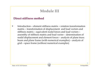
![1. Plane truss member
Stiffness coefficients in local coordinates
1
3
2 4
y
0 0
Degrees of freedom
1
⎛ ⎞
⎜ ⎟
Unit displacement
xEA
L
EA
L
⎜ ⎟
⎝ ⎠corr. to DOF 1
0 0
EA EA⎡ ⎤
−⎢ ⎥
[ ]
0 0
0 0 0 0
0 0
M
L L
S
EA EA
⎢ ⎥
⎢ ⎥
⎢ ⎥
⎢ ⎥
−⎢ ⎥
=
Member stiffness matrix in local
coordinates
Dept. of CE, GCE Kannur Dr.RajeshKN
0 0 0 0
L L
⎢ ⎥
⎢
⎢⎣ ⎦
⎥
⎥](https://image.slidesharecdn.com/module3-directstiffness-rajeshsir-140806045935-phpapp02/85/Module3-direct-stiffness-rajesh-sir-6-320.jpg)
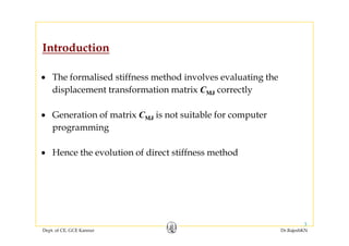
![Transformation of displacement vector
θ
Displacements in global
22 2 cosU D θ=
p g
coordinates: U1 and U2
Displacements in local
di D d D2D
DY iU D θ
12 2 sinU D θ= − θ
1 11 12 1 2cos sinU U U D Dθ θ= + = −
coordinates: D1 and D2
1DY
11 1 cosU D θ=
21 1 sinU D θ=
2 21 22 1 2sin cosU U U D Dθ θ= + = +
1 1cos sinU Dθ θ−⎧ ⎫ ⎧ ⎫⎡ ⎤
⎧ ⎫ ⎧ ⎫⎡ ⎤
1 1
2 2
cos sin
sin cos
U D
U D
θ θ
θ θ
⎧ ⎫ ⎧ ⎫⎡ ⎤
=⎨ ⎬ ⎨ ⎬⎢ ⎥
⎣ ⎦⎩ ⎭ ⎩ ⎭
X 1 1
2 2
cos sin
sin cos
D U
D U
θ θ
θ θ
⎧ ⎫ ⎧ ⎫⎡ ⎤
∴ =⎨ ⎬ ⎨ ⎬⎢ ⎥−⎣ ⎦⎩ ⎭ ⎩ ⎭
Dept. of CE, GCE Kannur Dr.RajeshKN
{ } [ ]{ }D R U=](https://image.slidesharecdn.com/module3-directstiffness-rajeshsir-140806045935-phpapp02/85/Module3-direct-stiffness-rajesh-sir-7-320.jpg)
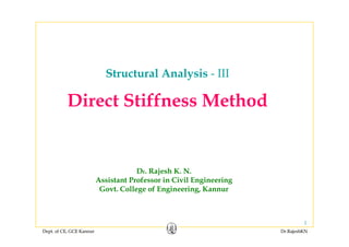
![C id i b th d
⎧ ⎫ ⎧ ⎫
Considering both ends,
1 1
2 2
cos sin 0 0
sin cos 0 0
0 0 i
D U
D U
D U
θ θ
θ θ
θ θ
⎧ ⎫ ⎧ ⎫⎡ ⎤
⎪ ⎪ ⎪ ⎪⎢ ⎥−⎪ ⎪ ⎪ ⎪⎢ ⎥=⎨ ⎬ ⎨ ⎬
⎢ ⎥3 3
4 4
0 0 cos sin
0 0 sin cos
D U
D U
θ θ
θ θ
⎨ ⎬ ⎨ ⎬
⎢ ⎥⎪ ⎪ ⎪ ⎪
⎢ ⎥⎪ ⎪ ⎪ ⎪−⎩ ⎭ ⎣ ⎦ ⎩ ⎭
{ } [ ]{ }LOCAL T GLOBALD R D=
[ ] [ ]R O⎡ ⎤
[ ]
[ ] [ ]
[ ] [ ]T
R O
R
O R
⎡ ⎤
= ⎢ ⎥
⎣ ⎦
Rotation matrix
Dept. of CE, GCE Kannur Dr.RajeshKN](https://image.slidesharecdn.com/module3-directstiffness-rajeshsir-140806045935-phpapp02/85/Module3-direct-stiffness-rajesh-sir-8-320.jpg)
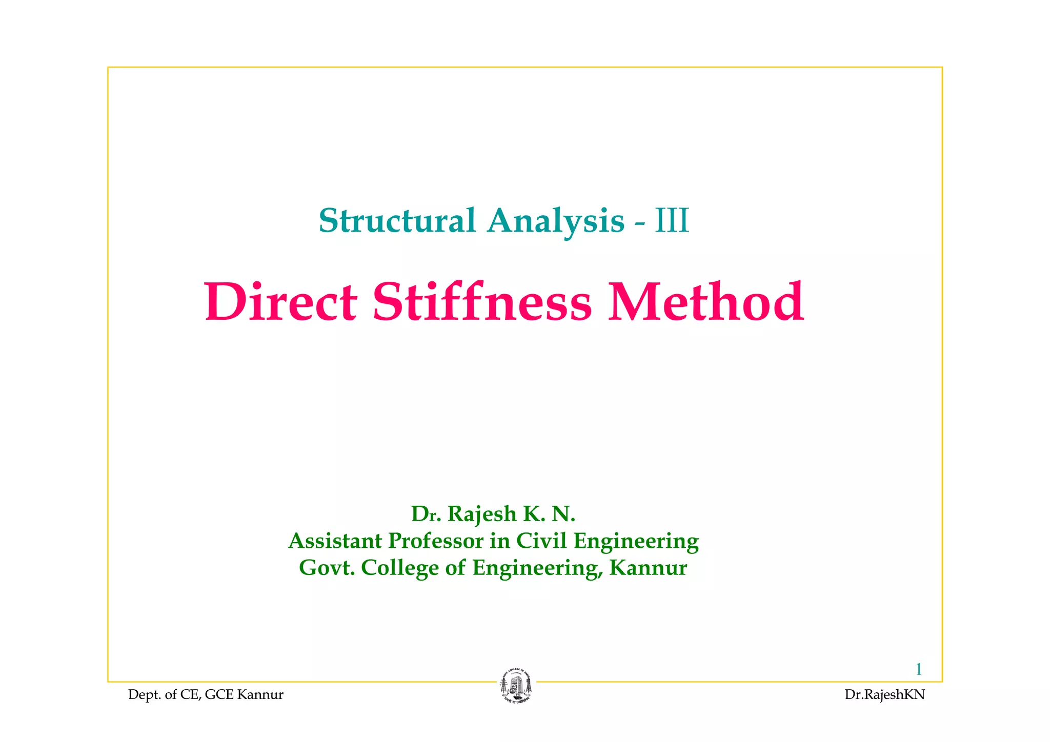
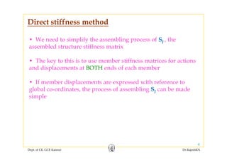
![Transformation of load vector Actions in global
θ
coordinates:
F1 and F2
22 2 cosF A θ= 1 11 12 1 2cos sinF F F A Aθ θ= + = −
22 2
12 2 sinF A θ= − θ 2A 2 21 22 1 2sin cosF F F A Aθ θ= + = +
Y
11 1 cosF A θ=
21 1 sinF A θ=1A 1 1
2 2
cos sin
sin cos
F A
F A
θ θ
θ θ
−⎧ ⎫ ⎧ ⎫⎡ ⎤
=⎨ ⎬ ⎨ ⎬⎢ ⎥
⎣ ⎦⎩ ⎭ ⎩ ⎭
11 1
1 1cos sinA Fθ θ⎧ ⎫ ⎧ ⎫⎡ ⎤
=⎨ ⎬ ⎨ ⎬⎢ ⎥
X
2 2sin cosA Fθ θ
⎨ ⎬ ⎨ ⎬⎢ ⎥−⎩ ⎭ ⎣ ⎦ ⎩ ⎭
{ } [ ]{ }A R F=
Dept. of CE, GCE Kannur Dr.RajeshKN
{ } [ ]{ }A R F=](https://image.slidesharecdn.com/module3-directstiffness-rajeshsir-140806045935-phpapp02/85/Module3-direct-stiffness-rajesh-sir-9-320.jpg)
![C id i b th dConsidering both ends,
1 1
2 2
cos sin 0 0
sin cos 0 0
A F
A F
θ θ
θ θ
⎧ ⎫ ⎧ ⎫⎡ ⎤
⎪ ⎪ ⎪ ⎪⎢ ⎥−⎪ ⎪ ⎪ ⎪⎢ ⎥=⎨ ⎬ ⎨ ⎬
3 3
4 4
0 0 cos sin
0 0 sin cos
A F
A F
θ θ
θ θ
⎢ ⎥=⎨ ⎬ ⎨ ⎬
⎢ ⎥⎪ ⎪ ⎪ ⎪
⎢ ⎥⎪ ⎪ ⎪ ⎪−⎩ ⎭ ⎣ ⎦ ⎩ ⎭
{ } [ ]{ }LOCAL T GLOBALi.e., A R A=
Dept. of CE, GCE Kannur Dr.RajeshKN
10](https://image.slidesharecdn.com/module3-directstiffness-rajeshsir-140806045935-phpapp02/85/Module3-direct-stiffness-rajesh-sir-10-320.jpg)
![Transformation of stiffness matrix
{ } [ ]{ }LOCAL M LOCALA S D=
[ ]{ } [ ][ ]{ }T GLOBAL M T GLOBALR A S R D=
{ } [ ] [ ][ ]{ }
1
GLOBAL T M T GLOBALA R S R D
−
=
[ ]{ } [ ][ ]{ }T GLOBAL M T GLOBAL
[ ] [ ]1 T
R R
−{ } [ ] [ ][ ]{ }GLOBAL T M T GLOBAL
{ } [ ]{ }A S D
[ ] [ ]T TR R=
{ } [ ]{ }GLOBAL MS GLOBALA S D=
[ ] [ ] [ ][ ]
T
MS T M TS R S R=where,
Member stiffness matrix in
global coordinates
Dept. of CE, GCE Kannur Dr.RajeshKN](https://image.slidesharecdn.com/module3-directstiffness-rajeshsir-140806045935-phpapp02/85/Module3-direct-stiffness-rajesh-sir-11-320.jpg)
![[ ] [ ] [ ][ ]
T
S R S R=
T
⎡ ⎤ ⎡ ⎤ ⎡ ⎤
[ ] [ ] [ ][ ]MS T M TS R S R=
0 0 1 0 1 0 0 0
0 0 0 0 0 0 0 0
T
c s c s
s c s cEA
−⎡ ⎤ ⎡ ⎤ ⎡ ⎤
⎢ ⎥ ⎢ ⎥ ⎢ ⎥− −
⎢ ⎥ ⎢ ⎥ ⎢ ⎥=
⎢ ⎥ ⎢ ⎥ ⎢ ⎥0 0 1 0 1 0 0 0
0 0 0 0 0 0 0 0
c s c sL
s c s c
−⎢ ⎥ ⎢ ⎥ ⎢ ⎥
⎢ ⎥ ⎢ ⎥ ⎢ ⎥
− −⎣ ⎦ ⎣ ⎦ ⎣ ⎦
2 2
c cs c cs⎡ ⎤− −
⎢ ⎥ M b tiff t i2 2
2 2
cs s cs sEA
L c cs c cs
⎢ ⎥
− −⎢ ⎥=
⎢ ⎥− −
⎢ ⎥
Member stiffness matrix
in global coordinates
for a plane truss member
2 2
cs s cs s
⎢ ⎥
− −⎣ ⎦
p
Dept. of CE, GCE Kannur Dr.RajeshKN
12](https://image.slidesharecdn.com/module3-directstiffness-rajeshsir-140806045935-phpapp02/85/Module3-direct-stiffness-rajesh-sir-12-320.jpg)
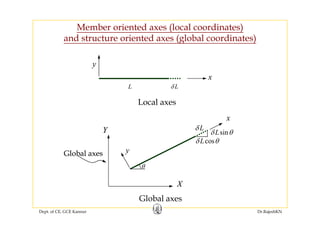
![2. Plane frame member
Stiffness coefficients in local coordinates
2 52
4
5
Degrees of freedom0 0 0 0
EA EA⎡ ⎤
1
3
4
6
Degrees of freedom
3 2 3 2
0 0 0 0
12 6 12 6
0 0
L L
EI EI EI EI
L L L L
⎡ ⎤
−⎢ ⎥
⎢ ⎥
⎢ ⎥−
⎢ ⎥
⎢ ⎥
[ ]
2 2
6 4 6 2
0 0
0 0 0 0
Mi
EI EI EI EI
L L L L
S
EA EA
⎢ ⎥
⎢ ⎥−
⎢ ⎥=
⎢ ⎥
−⎢ ⎥
Member stiffness matrix
in local coordinates
3 2 3 2
0 0 0 0
12 6 12 6
0 0
L L
EI EI EI EI
L L L L
−⎢ ⎥
⎢ ⎥
⎢ ⎥
− − −⎢ ⎥
⎢ ⎥
Dept. of CE, GCE Kannur Dr.RajeshKN
2 2
6 2 6 4
0 0
EI EI EI EI
L L L L
⎢ ⎥
⎢ ⎥−
⎢ ⎥⎣ ⎦](https://image.slidesharecdn.com/module3-directstiffness-rajeshsir-140806045935-phpapp02/85/Module3-direct-stiffness-rajesh-sir-13-320.jpg)
![Transformation of displacement vector
1 1
2 2
cos sin 0 0 0 0
sin cos 0 0 0 0
D U
D U
θ θ
θ θ
⎧ ⎫ ⎧ ⎫⎡ ⎤
⎪ ⎪ ⎪ ⎪⎢ ⎥−
⎪ ⎪ ⎪ ⎪⎢ ⎥
3 3
4 4
0 0 1 0 0 0
0 0 0 cos sin 0
D U
D Uθ θ
⎪ ⎪ ⎪ ⎪⎢ ⎥
⎪ ⎪ ⎪ ⎪⎢ ⎥
=⎨ ⎬ ⎨ ⎬⎢ ⎥
⎪ ⎪ ⎪ ⎪⎢ ⎥
⎪ ⎪ ⎪ ⎪⎢ ⎥5 5
6 6
0 0 0 sin cos 0
0 0 0 0 0 1
D U
D U
θ θ⎪ ⎪ ⎪ ⎪⎢ ⎥−
⎪ ⎪ ⎪ ⎪⎢ ⎥
⎣ ⎦⎩ ⎭ ⎩ ⎭
{ } [ ]{ }LOCAL T GLOBALD R D=
[ ] [ ]R O⎡ ⎤
{ } [ ]{ }LOCAL T GLOBAL
[ ]
[ ] [ ]
[ ] [ ]T
R O
R
O R
⎡ ⎤
= ⎢ ⎥
⎣ ⎦
Rotation matrix
Dept. of CE, GCE Kannur Dr.RajeshKN](https://image.slidesharecdn.com/module3-directstiffness-rajeshsir-140806045935-phpapp02/85/Module3-direct-stiffness-rajesh-sir-14-320.jpg)
![Transformation of load vector
{ } [ ]{ }LOCAL T GLOBALA R A={ } [ ]{ }
cos sin 0 0 0 0θ θ⎡ ⎤
⎢ ⎥
[ ]
sin cos 0 0 0 0
0 0 1 0 0 0
R
θ θ⎢ ⎥−
⎢ ⎥
⎢ ⎥
= ⎢ ⎥[ ]
0 0 0 cos sin 0
0 0 0 sin cos 0
TR
θ θ
θ θ
= ⎢ ⎥
⎢ ⎥
⎢ ⎥−
⎢ ⎥
0 0 0 0 0 1
⎢ ⎥
⎣ ⎦
Dept. of CE, GCE Kannur Dr.RajeshKN](https://image.slidesharecdn.com/module3-directstiffness-rajeshsir-140806045935-phpapp02/85/Module3-direct-stiffness-rajesh-sir-15-320.jpg)
![Transformation of stiffness matrix
{ } [ ]{ }GLOBAL MS GLOBALA S D=
[ ] [ ] [ ][ ]T
MS T M TS R S R= Member stiffness matrix in
global coordinatesglobal coordinates
EA EA⎡ ⎤
0 0 0 0
0 0 0 0
c s
s c
⎡ ⎤
⎢ ⎥−
⎢ ⎥
3 2 3 2
0 0 0 0
12 6 12 6
0 0
EA EA
L L
EI EI EI EI
L L L L
⎡ ⎤
−⎢ ⎥
⎢ ⎥
⎢ ⎥−
⎢ ⎥
⎢ ⎥
[ ]
0 0 1 0 0 0
0 0 0 0
0 0 0 0
T
c s
s c
R
⎢ ⎥
⎢ ⎥
= ⎢ ⎥
⎢ ⎥
⎢ ⎥−
⎢ ⎥
[ ]
2 2
6 4 6 2
0 0
0 0 0 0
M
EI EI EI EI
L L L LS
EA EA
L L
⎢ ⎥
⎢ ⎥−
⎢ ⎥=
⎢ ⎥
−⎢ ⎥
Where,
,
0 0 0 0 0 1
⎢ ⎥
⎣ ⎦
3 2 3 2
12 6 12 6
0 0
6 2 6 4
0 0
L L
EI EI EI EI
L L L L
EI EI EI EI
⎢ ⎥
⎢ ⎥
⎢ ⎥− − −⎢ ⎥
⎢ ⎥
⎢ ⎥
Dept. of CE, GCE Kannur Dr.RajeshKN
2 2
0 0
L L L L
⎢ ⎥−
⎢ ⎥⎣ ⎦](https://image.slidesharecdn.com/module3-directstiffness-rajeshsir-140806045935-phpapp02/85/Module3-direct-stiffness-rajesh-sir-16-320.jpg)
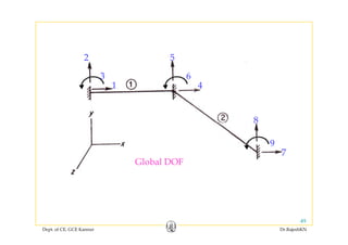
![1 2 3 4
Global DOF
11 12 13 14
1 1 1 1
21 22 23 24
2 2
2 2
1
2
M M M M
s s s s
s s s s
c cs c cs
cs s cs sEA
− −⎡ ⎤ ⎡ ⎤
⎢ ⎥ ⎢ ⎥− −
⎢ ⎥ ⎢ ⎥
1 2 3 4
[ ] 1 1 1 1
31 32 33 34
1 1 1 1
41 42 43 44
1 2 2
2 2
2
3
4
M M M M
M M M M
M
s s s s
s s s s
cs s cs sEA
S
c cs c csL
− −
⎢ ⎥ ⎢ ⎥= =
− −⎢ ⎥ ⎢ ⎥
⎢ ⎥ ⎢ ⎥
⎣ ⎦⎣ ⎦
41 42 43 44
1 1 1 1
2 2
4M M M M
s s s scs s cs s
⎢ ⎥ ⎢ ⎥− − ⎣ ⎦⎣ ⎦
1 2 3 4 5 6
1
2
× × × ×⎡ ⎤
⎢ ⎥× × × ×
⎢ ⎥ C t ib ti f
[ ]
2
3
4
JS
× × × ×
⎢ ⎥
× × × ×⎢ ⎥
= ⎢ ⎥
Contribution of
Member 1 to global
stiffness matrix[ ]
4
5
J ⎢ ⎥
× × × ×⎢ ⎥
⎢ ⎥
⎢ ⎥
Dept. of CE, GCE Kannur Dr.RajeshKN
6
⎢ ⎥
⎣ ⎦](https://image.slidesharecdn.com/module3-directstiffness-rajeshsir-140806045935-phpapp02/85/Module3-direct-stiffness-rajesh-sir-19-320.jpg)
![3 4 5 6
Global DOF
11 12 13 14
2 2 2 2
21 22 23 24
3
4
M M M M
s s s s
s s s s
⎡ ⎤
⎢ ⎥
⎢ ⎥
3 4 5 6
[ ] 2 2
2
2 2
31 32 33 34
2 2 2 2
41 42 43 44
4
5
6
M M M M
M M M
M
M
s s s s
s s s s
s s s s
S = ⎢ ⎥
⎢ ⎥
⎢ ⎥
⎣ ⎦2 2 2 2
6M M M M
s s s s⎣ ⎦
1 2 3 4 5 6
1
2
⎡ ⎤
⎢ ⎥
⎢ ⎥ C t ib ti f
[ ]
2
3
4
JS
⎢ ⎥
× × × ×⎢ ⎥
= ⎢ ⎥
× × × ×⎢ ⎥
Contribution of
Member 2 to global
stiffness matrix
4
5
6
× × × ×⎢ ⎥
⎢ ⎥× × × ×
⎢ ⎥
⎣ ⎦
Dept. of CE, GCE Kannur Dr.RajeshKN
6
⎢ ⎥
× × × ×⎣ ⎦](https://image.slidesharecdn.com/module3-directstiffness-rajeshsir-140806045935-phpapp02/85/Module3-direct-stiffness-rajesh-sir-20-320.jpg)
![11 12 13 14
1⎡ ⎤
1 2 5 6
Global DOF
[ ]
11 12 13 14
3 3 3 3
21 22 23 24
3 3 3 3
1
2
M M M M
M M M M
s s s s
s s s s
S
⎡ ⎤
⎢ ⎥
⎢ ⎥[ ] 3 3
3
3 3
31 32 33 34
3 3 3 3
41 42 43 44
5
6
M M M M
M M M
M
M
s s s s
S = ⎢ ⎥
⎢ ⎥
⎢ ⎥
⎣ ⎦
41 42 43 44
3 3 3 3
6M M M M
s s s s
⎢ ⎥
⎣ ⎦
1 2 3 4 5 6
1
2
× × × ×⎡ ⎤
⎢ ⎥
1 2 3 4 5 6
[ ]
2
3
JS
⎢ ⎥× × × ×
⎢ ⎥
⎢ ⎥
= ⎢ ⎥
Contribution of
Member 3 to global
stiffness matrix[ ]
4
5
JS ⎢ ⎥
⎢ ⎥
⎢ ⎥× × × ×
⎢ ⎥
stiffness matrix
Dept. of CE, GCE Kannur Dr.RajeshKN
6
⎢ ⎥
× × × ×⎣ ⎦](https://image.slidesharecdn.com/module3-directstiffness-rajeshsir-140806045935-phpapp02/85/Module3-direct-stiffness-rajesh-sir-21-320.jpg)
![Assembled global stiffness matrix
11 12 13 1411 12 13 14
s s s ss s s s+ + 1⎡ ⎤
1 2 3 4 5 6
1 1 1 1
21 22 23 24
1 1 1 1
3 3 3 3
21 22 23 24
3 3 3 3
M M M M
M M M M
M M M M
M M M M
s s s s
s s s s
s s s s
s s s s
+ +
+ +
1
2
⎡ ⎤
⎢ ⎥
⎢ ⎥
⎢ ⎥
[ ]
31 32 3 11 12 13 14
2 2 2 2
21 22 23 24
3 34
1 1 1 1
41 42 43 44
M M M MM M M M
J
s s s s
s s s s
s s s s
s
S
ss s
+ +
=
+ +
3
4
⎢ ⎥
⎢ ⎥
⎢ ⎥
31 3
2 2 2 2
31 32 33
1 1
2
2
1 1
23 3 32
M M M M
M MM M
M M M M
MM
s s
s s s s
s s
s s
s
s s
s
+ +
+
34
2
33 34
3
4
5MM
ss +
⎢ ⎥
⎢ ⎥
⎢ ⎥41 42 43 44
2
41 42 43 44
3 2 23 32 3
6M M M MM M M M
s s s ss s s s+ +
⎢ ⎥
⎣ ⎦
Dept. of CE, GCE Kannur Dr.RajeshKN](https://image.slidesharecdn.com/module3-directstiffness-rajeshsir-140806045935-phpapp02/85/Module3-direct-stiffness-rajesh-sir-22-320.jpg)
![Reduced equation systemq y
(after imposing boundary conditions)
33 34
1 1
43 44
11 12
2 2
21 22
3 3MM M M
F U
F U
s ss s+ +⎧ ⎫ ⎧ ⎫⎡ ⎤
=⎨ ⎬ ⎨ ⎬⎢ ⎥+ +⎩ ⎭ ⎣ ⎦⎩ ⎭1 2 1 24 4M MM M
F Us sss⎢ ⎥+ +⎩ ⎭ ⎣ ⎦⎩ ⎭
•This reduced equation system can be solved to get the unknown
displacement components 3 4
,U U
{ } [ ]{ }LOCAL T GLOBALD R D=•From
{ }LOCALD can be found out.
{ } { }D D=F h b
Dept. of CE, GCE Kannur Dr.RajeshKN
{ } { }LOCAL MiD D=•For each member,](https://image.slidesharecdn.com/module3-directstiffness-rajeshsir-140806045935-phpapp02/85/Module3-direct-stiffness-rajesh-sir-24-320.jpg)
![{ } { } [ ]{ }A A S D{ } { } [ ]{ }Mi MLi Mi MiA A S D= +Member end actions
Where,
Fixed end actions on the member,{ }MLiA
Member stiffness matrix,[ ]MiS
[ ]
in local
coordinates
Displacement components of the member,[ ]MiD
{ } { } [ ]{ }LOCAL T GLOBALMi D R DD ==As we know,
{ } { } [ ][ ]{ }i i iM ML M i iT GLOBALA A S R D∴ = +
Dept. of CE, GCE Kannur Dr.RajeshKN
25](https://image.slidesharecdn.com/module3-directstiffness-rajeshsir-140806045935-phpapp02/85/Module3-direct-stiffness-rajesh-sir-25-320.jpg)
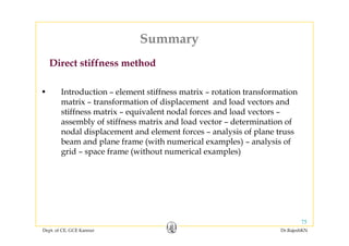
![Direct Stiffness Method: Procedure
STEP 1: Get member stiffness matrices for all members [ ]MiS
STEP 2: Get rotation matrices for all members
[ ]TiR
STEP 3: Transform member stiffness matrices from local coordinates
into global coordinates to get [ ]MSiS[ ]MSi
STEP 4: Assemble global stiffness matrix [ ]JS
STEP 5: Impose boundary conditions to get the reduced stiffness
matrix [ ]S[ ]FFS
Dept. of CE, GCE Kannur Dr.RajeshKN
26](https://image.slidesharecdn.com/module3-directstiffness-rajeshsir-140806045935-phpapp02/85/Module3-direct-stiffness-rajesh-sir-26-320.jpg)
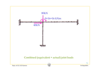
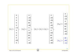
![STEP 6: Find equivalent joint loads from applied loads on eachq j pp
member (loads other than those applied at joints directly)
STEP 7 T f b ti f l l di t i t l b lSTEP 7: Transform member actions from local coordinates into global
coordinates to get the transformed load vector
STEP 8: Find combined load vector by adding the above
transformed load vector and the loads applied directly at joints
[ ]CA
STEP 9: Find the reduced load vector by removing members in
h l d di b d di i
[ ]FCA
the load vector corresponding to boundary conditions
STEP 10: Get displacement components of the structure in global
coordinates { } [ ] { }
1
F FF FCD S A
−
=
Dept. of CE, GCE Kannur Dr.RajeshKN
27](https://image.slidesharecdn.com/module3-directstiffness-rajeshsir-140806045935-phpapp02/85/Module3-direct-stiffness-rajesh-sir-27-320.jpg)
![{ } [ ]{ }LOCAL T GLOBALD R D=
STEP 11: Get displacement components of each member in local
coordinates
STEP 12: Get member end actions from
{ } { } [ ][ ]{ }Mi MLi Mi iT GLOB iALR DA A S∴ = +
{ } { } [ ][ ]R RC RF FA A S D= − +STEP 13: Get reactions from
{ }RCA represents combined joint loads (actual and
equivalent) applied directly to the supports.q ) pp y pp
Dept. of CE, GCE Kannur Dr.RajeshKN
28](https://image.slidesharecdn.com/module3-directstiffness-rajeshsir-140806045935-phpapp02/85/Module3-direct-stiffness-rajesh-sir-28-320.jpg)
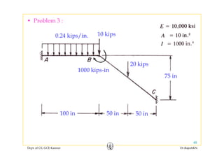
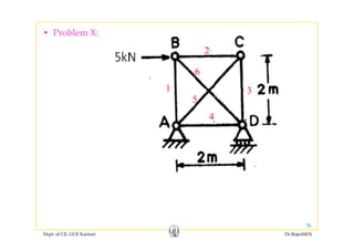
![• Problem 1:
1 Member stiffness matrices in local co ordinates
1EA ⎡ ⎤⎡ ⎤
1. Member stiffness matrices in local co-ordinates
(without considering restraint DOF)
[ ]1
1
00
1.155
0 0 0 0
M
EA
S L
⎡ ⎤⎡ ⎤
⎢ ⎥⎢ ⎥= =
⎢ ⎥⎢ ⎥
⎣ ⎦ ⎣ ⎦0 0 0 0⎣ ⎦ ⎣ ⎦
[ ]
1 0⎡ ⎤
[ ]
1 2 0⎡ ⎤
Dept. of CE, GCE Kannur Dr.RajeshKN
[ ]2
1 0
0 0
MS
⎡ ⎤
= ⎢ ⎥
⎣ ⎦
[ ]3
1 2 0
0 0MS
⎡ ⎤
= ⎢ ⎥
⎣ ⎦](https://image.slidesharecdn.com/module3-directstiffness-rajeshsir-140806045935-phpapp02/85/Module3-direct-stiffness-rajesh-sir-29-320.jpg)
![2. Rotation (transformation) matrices
[ ]1
cos sin 0.5 0.866
i 0 866 0 5
TR
θ θ
θ θ
−⎡ ⎤ ⎡ ⎤
= =⎢ ⎥ ⎢ ⎥
⎣ ⎦ ⎣ ⎦
[ ]1
60 sin cos 0.866 0.5
T
θ θ θ=−
⎢ ⎥ ⎢ ⎥−⎣ ⎦ ⎣ ⎦
[ ]2
90
0 1
1 0
TR
θ
−⎡ ⎤
= ⎢ ⎥
⎣ ⎦90 1 0θ =− ⎣ ⎦
[ ]3
150
0.866 0.5
0.5 0.866
TR
θ =−
− −⎡ ⎤
= ⎢ ⎥−⎣ ⎦⎣ ⎦
Dept. of CE, GCE Kannur Dr.RajeshKN
30](https://image.slidesharecdn.com/module3-directstiffness-rajeshsir-140806045935-phpapp02/85/Module3-direct-stiffness-rajesh-sir-30-320.jpg)
![3. Member stiffness matrices in global co-ordinates
(Transformed member stiffness matrices)
[ ] [ ] [ ][ ]1 1 1 1
T
MS T M TS R S R=
0.5 0.866 1 0 0.5 0.8661
0 866 0 5 0 0 0 866 0 51 155
T
− −⎡ ⎤ ⎡ ⎤ ⎡ ⎤
= ⎢ ⎥ ⎢ ⎥ ⎢ ⎥
⎣ ⎦ ⎣ ⎦ ⎣ ⎦0.866 0.5 0 0 0.866 0.51.155⎢ ⎥ ⎢ ⎥ ⎢ ⎥
⎣ ⎦ ⎣ ⎦ ⎣ ⎦
0 216 0 375−⎡ ⎤0.216 0.375
0.375 0.649
−⎡ ⎤
= ⎢ ⎥−⎣ ⎦
Dept. of CE, GCE Kannur Dr.RajeshKN](https://image.slidesharecdn.com/module3-directstiffness-rajeshsir-140806045935-phpapp02/85/Module3-direct-stiffness-rajesh-sir-31-320.jpg)
![[ ]2
0 1 1 0 0 1
1 0 0 0 1 0
T
MSS
− −⎡ ⎤ ⎡ ⎤ ⎡ ⎤
= ⎢ ⎥ ⎢ ⎥ ⎢ ⎥
⎣ ⎦ ⎣ ⎦ ⎣ ⎦⎣ ⎦ ⎣ ⎦ ⎣ ⎦
0 0⎡ ⎤
= ⎢ ⎥0 1
= ⎢ ⎥
⎣ ⎦
[ ]3
0.866 0.5 1 0 0.866 0.51
0 5 0 866 0 0 0 5 0 8662
T
MSS
− − − −⎡ ⎤ ⎡ ⎤ ⎡ ⎤
= ⎢ ⎥ ⎢ ⎥ ⎢ ⎥
⎣ ⎦ ⎣ ⎦ ⎣ ⎦
[ ]3
0.5 0.866 0 0 0.5 0.8662
MS ⎢ ⎥ ⎢ ⎥ ⎢ ⎥− −⎣ ⎦ ⎣ ⎦ ⎣ ⎦
0.375 0.217⎡ ⎤
⎢ ⎥0.217 0.125
= ⎢ ⎥
⎣ ⎦
Dept. of CE, GCE Kannur Dr.RajeshKN
32](https://image.slidesharecdn.com/module3-directstiffness-rajeshsir-140806045935-phpapp02/85/Module3-direct-stiffness-rajesh-sir-32-320.jpg)
![4. Global stiffness matrix
0 216 0 0 375 0 375 0 0 217⎡ ⎤
(by assembling transformed member stiffness matrices)
[ ]
0.216 0 0.375 0.375 0 0.217
0.375 0 0.217 0.649 1 0.125
FFS
+ + − + +⎡ ⎤
= ⎢ ⎥− + + + +⎣ ⎦
0.591 0.158
0 158 1 774
−⎡ ⎤
= ⎢ ⎥
⎣ ⎦0.158 1.774⎢ ⎥−⎣ ⎦
This is the reduced global stiffness matrix, since restraint DOF
were not considered. Hence, boundary conditions are
automatically incorporatedautomatically incorporated.
Dept. of CE, GCE Kannur Dr.RajeshKN](https://image.slidesharecdn.com/module3-directstiffness-rajeshsir-140806045935-phpapp02/85/Module3-direct-stiffness-rajesh-sir-33-320.jpg)
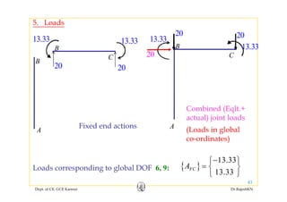
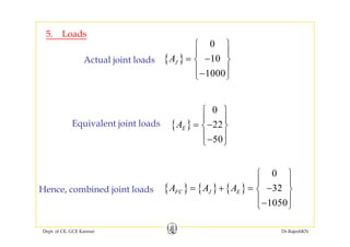
![5. Loads
{ }
0
5
FCA
⎧ ⎫
= ⎨ ⎬
−⎩ ⎭
6. Joint displacements6. Joint displacements
0 772⎧ ⎫
{ } [ ] { }
1
F FF FCD S A
−
=
0.772
2.89
−⎧ ⎫
= ⎨ ⎬
−⎩ ⎭
Dept. of CE, GCE Kannur Dr.RajeshKN
34](https://image.slidesharecdn.com/module3-directstiffness-rajeshsir-140806045935-phpapp02/85/Module3-direct-stiffness-rajesh-sir-34-320.jpg)
![7. Member forces
{ } { } [ ][ ]{ }Mi MLi Mi iT GLOB iALR DA A S∴ = +
Member 1
{ } { } [ ][ ]{ }
{ } { } [ ][ ]{ }1 1 1 1 1TM M G LM L BAL OR DA A S= + [ ][ ]{ }1 1 1T GLOBALM R DS=
1
0.5 0.8660
1 155
0.772⎡ ⎤ −⎡ ⎤⎢ ⎥= ⎢ ⎥⎢
−⎧
⎥
⎫
⎨ ⎬
1.833
=
⎧ ⎫
⎨ ⎬1.155
0.866 0.5
0 0
2.89⎢ ⎥⎢ ⎥ ⎣ ⎦
⎣ ⎦
⎨ ⎬
−⎩ ⎭ 0
⎨ ⎬
⎩ ⎭
Dept. of CE, GCE Kannur Dr.RajeshKN
35](https://image.slidesharecdn.com/module3-directstiffness-rajeshsir-140806045935-phpapp02/85/Module3-direct-stiffness-rajesh-sir-35-320.jpg)
![{ } [ ][ ]{ }R DA SM b 2 { } [ ][ ]{ }2 2 2 2T GLOBALM M R DA S=Member 2
0.772
2
1 0 0 1
0 0 1 0 .89
−⎡ ⎤ ⎡ ⎤
= ⎢ ⎥ ⎢ ⎥
⎣ ⎦
−⎧ ⎫
⎨
⎦ −⎩⎣
⎬
⎭
2.89
0
⎧
=
⎫
⎨ ⎬
⎩ ⎭
Member 3
{ } [ ][ ]{ }3 3 3 3T GLOBALM M R DA S=
1 2 0 0.866 0.5
0 0 0.5 0.866
0.772
2.89
− −⎡ ⎤ ⎡ ⎤
= ⎢ ⎥ ⎢ ⎥−⎣ ⎦
−⎧ ⎫
⎨
⎣ ⎦
⎬
−⎩ ⎭
1.057
0
=
⎧ ⎫
⎨ ⎬
⎩ ⎭⎣ ⎦ ⎣ ⎦ ⎩ ⎭ ⎩ ⎭
Dept. of CE, GCE Kannur Dr.RajeshKN
36](https://image.slidesharecdn.com/module3-directstiffness-rajeshsir-140806045935-phpapp02/85/Module3-direct-stiffness-rajesh-sir-36-320.jpg)
![0 0 0 0
12 6 12 6
EA EA
L L
EI EI EI EI
⎡ ⎤
−⎢ ⎥
⎢ ⎥
⎢ ⎥
3 2 3 2
2 2
12 6 12 6
0 0
6 4 6 2
0 0
EI EI EI EI
L L L L
EI EI EI EI
L L L L
⎢ ⎥
⎢ ⎥−
⎢ ⎥
⎢ ⎥
⎢ ⎥−
⎢ ⎥
Member stiffness matrix
[ ]
0 0 0 0
12 6 12 6
Mi
L L L LS
EA EA
L L
EI EI EI EI
⎢ ⎥=
⎢ ⎥
−⎢ ⎥
⎢ ⎥
⎢ ⎥
of a 2D frame member in
local coordinates
3 2 3 2
2 2
12 6 12 6
0 0
6 2 6 4
0 0
EI EI EI EI
L L L L
EI EI EI EI
L L L L
⎢ ⎥− − −⎢ ⎥
⎢ ⎥
⎢ ⎥−
⎢ ⎥⎣ ⎦L L L L⎢ ⎥⎣ ⎦
Dept. of CE, GCE Kannur Dr.RajeshKN
39](https://image.slidesharecdn.com/module3-directstiffness-rajeshsir-140806045935-phpapp02/85/Module3-direct-stiffness-rajesh-sir-39-320.jpg)
![1. Member stiffness matrices in local co-ordinates
( ith t id i t i t DOF)
6Local DOFMember 1
(without considering restraint DOF)
[ ] 4EI
S ⎡ ⎤=
⎢ ⎥ [ ]1EI EI= =
6Global DOF
[ ]1MS
L
=
⎢ ⎥⎣ ⎦
[ ]1EI EI
Member 2
6 9Global DOF
3 6Local DOF
Member 2
[ ]
4 2EI EI
L LS
⎡ ⎤
⎢ ⎥
⎢ ⎥
6 9Global DOF
0.5EI EI⎡ ⎤
[ ]2
2 4
M
L LS
EI EI
L L
= ⎢ ⎥
⎢ ⎥
⎢ ⎥⎣ ⎦
0.5EI EI
⎡ ⎤
= ⎢ ⎥
⎣ ⎦
Dept. of CE, GCE Kannur Dr.RajeshKN
40](https://image.slidesharecdn.com/module3-directstiffness-rajeshsir-140806045935-phpapp02/85/Module3-direct-stiffness-rajesh-sir-40-320.jpg)
![2. Rotation (transformation) matrices
In this case, transformation matrices are:
[ ] [ ]1 1TR = corresponding to local DOF 6
[ ]2
1 0
0 1
TR
⎡ ⎤
= ⎢ ⎥
⎣ ⎦
corresponding to local DOFs 3 & 6
⎣ ⎦
3. Member stiffness matrices in global co-ordinates
(Transformed member stiffness matrices)
[ ]1MSS EI= [ ]2
0.5
0.5
MS
EI EI
S
EI EI
⎡ ⎤
= ⎢ ⎥
⎣ ⎦
Dept. of CE, GCE Kannur Dr.RajeshKN
⎣ ⎦](https://image.slidesharecdn.com/module3-directstiffness-rajeshsir-140806045935-phpapp02/85/Module3-direct-stiffness-rajesh-sir-41-320.jpg)
![4 A bl d ( d d d) l b l tiff t i
6 9Gl b l DOF
4. Assembled (and reduced) global stiffness matrix
[ ]
0.5EI EI
S
IE⎡ + ⎤
= ⎢ ⎥
6 9Global DOF
2 0.5
EI
⎡ ⎤
= ⎢ ⎥[ ]
0.5FFS
EI EI
= ⎢ ⎥
⎣ ⎦ 0.5 1
EI= ⎢ ⎥
⎣ ⎦
Dept. of CE, GCE Kannur Dr.RajeshKN](https://image.slidesharecdn.com/module3-directstiffness-rajeshsir-140806045935-phpapp02/85/Module3-direct-stiffness-rajesh-sir-42-320.jpg)
![6 Joint displacements
11 431 ⎧ ⎫
6. Joint displacements
{ } [ ] { }
1
F FF FCD S A
−
=
11.43
19.04
1
EI
−⎧
=
⎫
⎨ ⎬
⎩ ⎭
Dept. of CE, GCE Kannur Dr.RajeshKN
44](https://image.slidesharecdn.com/module3-directstiffness-rajeshsir-140806045935-phpapp02/85/Module3-direct-stiffness-rajesh-sir-44-320.jpg)
![7. Member end actions
{ } { } [ ][ ]{ }Mi MLi Mi iT GLOB iALR DA A S∴ = +
: fixed end actions for member i{ }MLiA
Member 1
{ } { } [ ][ ]{ }1 1 1 1 1TM M G LM L BAL OR DA A S= +
{ } [ ]{ }DA S { } { }
4 1
0 11 43
EI⎡ ⎤
{ } [ ]{ }1 1 1ML M GLOBALDA S= + { } { }0 11.43
11.43
L EI
⎡ ⎤
= + −⎢ ⎥⎣ ⎦
= −
This is the member end action corresponding to local DOF 6
f M b 1 i b d h d f
Dept. of CE, GCE Kannur Dr.RajeshKN
45
of Member 1. i.e., member end moment at the top edge of
Member 1.](https://image.slidesharecdn.com/module3-directstiffness-rajeshsir-140806045935-phpapp02/85/Module3-direct-stiffness-rajesh-sir-45-320.jpg)
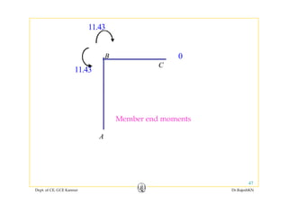
![Member 2
{ } { } [ ]{ }2 2 2 2M ML M GLOBALA A DS= +
Member 2
13.33 11.43
13.33 1
0.5
9.04
1
0.5
EI EI
EI EI EI
−⎧ ⎫ ⎧ ⎫
+
⎡ ⎤
= ⎢ ⎥
⎣
⎨ ⎬ ⎨
−⎩ ⎭ ⎩⎦
⎬
⎭
13.33 1.91−⎧ ⎫ ⎧ ⎫
+⎨ ⎬ ⎨= ⎬
11.42
=
⎧ ⎫
⎨ ⎬
Th th b ti di t l l DOF 3
13.33 13.325
+⎨ ⎬ ⎨
⎩ ⎭
⎬
− ⎩ ⎭ 0
⎨ ⎬
⎩ ⎭
These are the member actions corresponding to local DOFs 3
and 6 of Member 2. i.e., member end moments of Member 2.
Dept. of CE, GCE Kannur Dr.RajeshKN
46](https://image.slidesharecdn.com/module3-directstiffness-rajeshsir-140806045935-phpapp02/85/Module3-direct-stiffness-rajesh-sir-46-320.jpg)
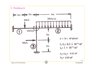
![1. Member stiffness matrices in local co-ordinates
( ith t id i t i t DOF)(without considering restraint DOF)
0 0
12 6
XEA
L
EI EI
⎡ ⎤
⎢ ⎥
⎢ ⎥
⎢ ⎥
1000 0 0⎡ ⎤
⎢ ⎥[ ]1 3 2
12 6
0
6 4
0
Z Z
M
Z Z
EI EI
S
L L
EI EI
⎢ ⎥= −
⎢ ⎥
⎢ ⎥
⎢ ⎥−
5
0 120 6000
0 6000 4 10
⎢ ⎥= −
⎢ ⎥
− ×⎢ ⎥⎣ ⎦
2
0
L L
⎢ ⎥−
⎣ ⎦
0 0
12 6
XEA
L
EI EI
⎡ ⎤
⎢ ⎥
⎢ ⎥
⎢ ⎥
800 0 0⎡ ⎤
⎢ ⎥
[ ]2 3 2
12 6
0
6 4
0
Z Z
M
Z Z
EI EI
S
L L
EI EI
⎢ ⎥=
⎢ ⎥
⎢ ⎥
⎢ ⎥
5
0 61.44 3840
0 3840 3.2 10
⎢ ⎥=
⎢ ⎥
×⎢ ⎥⎣ ⎦
Dept. of CE, GCE Kannur Dr.RajeshKN
52
2
0
L L
⎢ ⎥
⎣ ⎦](https://image.slidesharecdn.com/module3-directstiffness-rajeshsir-140806045935-phpapp02/85/Module3-direct-stiffness-rajesh-sir-52-320.jpg)
![2. Rotation (transformation) matrices
[ ]
cos sin 0
i 0R
⎡ ⎤
⎢ ⎥
θ θ
θ θ[ ] sin cos 0
0 0 1
TR ⎢ ⎥= −
⎢ ⎥
⎢ ⎥⎣ ⎦
θ θ
Member 1
Member 2
[ ]2
0.8 0.6 0
0.6 0.8 0R
−⎡ ⎤
⎢ ⎥=
⎢ ⎥[ ]1
1 0 0
0 1 0R
⎡ ⎤
⎢ ⎥=
⎢ ⎥
[ ]
0 0 1
⎢ ⎥
⎢ ⎥⎣ ⎦
[ ]1
0 0 1
⎢ ⎥
⎢ ⎥⎣ ⎦
Dept. of CE, GCE Kannur Dr.RajeshKN
53](https://image.slidesharecdn.com/module3-directstiffness-rajeshsir-140806045935-phpapp02/85/Module3-direct-stiffness-rajesh-sir-53-320.jpg)
![3. Member stiffness matrices in global co-ordinates
(Transformed member stiffness matrices)
[ ] [ ] [ ][ ]1 1 1 1
T
MS T M TS R S R=
1 0 0 1000 0 0 1 0 0
0 1 0 0 120 6000 0 1 0
T
⎡ ⎤ ⎡ ⎤ ⎡ ⎤
⎢ ⎥ ⎢ ⎥ ⎢ ⎥=
⎢ ⎥ ⎢ ⎥ ⎢ ⎥
5
0 1 0 0 120 6000 0 1 0
0 0 1 0 6000 4 10 0 0 1
= −
⎢ ⎥ ⎢ ⎥ ⎢ ⎥
− ×⎢ ⎥ ⎢ ⎥ ⎢ ⎥⎣ ⎦ ⎣ ⎦ ⎣ ⎦
5
1000 0 0
0 120 6000
⎡ ⎤
⎢ ⎥= −
⎢ ⎥
⎢ ⎥5
0 6000 4 10− ×⎢ ⎥⎣ ⎦
Dept. of CE, GCE Kannur Dr.RajeshKN
54](https://image.slidesharecdn.com/module3-directstiffness-rajeshsir-140806045935-phpapp02/85/Module3-direct-stiffness-rajesh-sir-54-320.jpg)
![[ ]
0.8 0.6 0 800 0 0 0.8 0.6 0
0 6 0 8 0 0 61 44 3840 0 6 0 8 0
T
S
− −⎡ ⎤ ⎡ ⎤ ⎡ ⎤
⎢ ⎥ ⎢ ⎥ ⎢ ⎥
[ ]2
5
0.6 0.8 0 0 61.44 3840 0.6 0.8 0
0 0 1 0 3840 3.2 10 0 0 1
MSS ⎢ ⎥ ⎢ ⎥ ⎢ ⎥=
⎢ ⎥ ⎢ ⎥ ⎢ ⎥
×⎢ ⎥ ⎢ ⎥ ⎢ ⎥⎣ ⎦ ⎣ ⎦ ⎣ ⎦
0.8 0.6 0 640 480 0
0 6 0 8 0 36 86 49 15 3840
−⎡ ⎤ ⎡ ⎤
⎢ ⎥ ⎢ ⎥= −
⎢ ⎥ ⎢ ⎥
5
0.6 0.8 0 36.86 49.15 3840
0 0 1 2304 3072 3.2 10
= −
⎢ ⎥ ⎢ ⎥
×⎢ ⎥ ⎢ ⎥⎣ ⎦ ⎣ ⎦
534.12 354.51 2304
354 51 327 32 3072
−⎡ ⎤
⎢ ⎥= −
⎢ ⎥
5
354.51 327.32 3072
2304 3072 3.2 10
⎢ ⎥
×⎢ ⎥⎣ ⎦
Dept. of CE, GCE Kannur Dr.RajeshKN](https://image.slidesharecdn.com/module3-directstiffness-rajeshsir-140806045935-phpapp02/85/Module3-direct-stiffness-rajesh-sir-55-320.jpg)
![4. Assembled (reduced) global stiffness matrix
1000 534.12 0 354.51 0 2304+ − +⎡ ⎤
. sse b ed ( educed) g oba st ess at x
[ ]
5 5
0 354.51 120 327.32 6000 3072
0 2304 6000 3072 4 10 3.2 10
FFS
⎡ ⎤
⎢ ⎥= − + − +
⎢ ⎥
+ − + × + ×⎢ ⎥⎣ ⎦0 2304 6000 3072 4 10 3.2 10+ + × + ×⎢ ⎥⎣ ⎦
1534 12 354 51 2304⎡ ⎤
5
1534.12 354.51 2304
354.51 447.32 2928
−⎡ ⎤
⎢ ⎥− −
⎢
⎢
=
⎥
⎥5
2304 2928 7.2 10− ×⎢⎣ ⎦⎥
Dept. of CE, GCE Kannur Dr.RajeshKN
56](https://image.slidesharecdn.com/module3-directstiffness-rajeshsir-140806045935-phpapp02/85/Module3-direct-stiffness-rajesh-sir-56-320.jpg)
![6. Joint displacements
{ } [ ] { }
1
F FF FCD S A
−
={ } [ ] { }F FF FCD S A
1
{ }
1
1534.12 354.51 2304 0
354.51 447.32 2928 32FD
−
− ⎧ ⎫⎡ ⎤
⎪ ⎪⎢ ⎥∴ = − − −⎨ ⎬⎢ ⎥
⎪ ⎪5
2304 2928 7.2 10 1050
⎢ ⎥
⎪ ⎪− × −⎢ ⎥ ⎩ ⎭⎣ ⎦
0.0206
0.09936
−⎧ ⎫
⎪ ⎪
= −⎨ ⎬0.09936
0.001797
⎨ ⎬
⎪ ⎪−⎩ ⎭
Dept. of CE, GCE Kannur Dr.RajeshKN](https://image.slidesharecdn.com/module3-directstiffness-rajeshsir-140806045935-phpapp02/85/Module3-direct-stiffness-rajesh-sir-58-320.jpg)
![7. Member end actions
{ } { } [ ][ ]{ }Mi MLi Mi iT GLOB iALR DA A S∴ = +
1000 0 0 1 0 0 0.0206⎡ ⎤ ⎡ ⎤ −⎧ ⎫
⎪ ⎪
{ }
5
0 120 6000 0 1 0 0.0993
0 6000 4 10 0
6
0 1 0.001797
MLiA
⎡ ⎤ ⎡ ⎤
⎢ ⎥ ⎢ ⎥= + −
⎢ ⎥ ⎢ ⎥
− ×⎢ ⎥ ⎢ ⎥
⎧ ⎫
⎪ ⎪
−⎨
⎣ ⎦ ⎣
⎪
⎩⎦
⎬
⎪− ⎭0 6000 4 10 0 0 1 0.001797⎢ ⎥ ⎢ ⎥⎣ ⎦ ⎣ ⎩⎦ ⎭
8. Reactions
{ } { } [ ][ ]R RC RF FA A S D= − +
Dept. of CE, GCE Kannur Dr.RajeshKN](https://image.slidesharecdn.com/module3-directstiffness-rajeshsir-140806045935-phpapp02/85/Module3-direct-stiffness-rajesh-sir-59-320.jpg)
![1. Member stiffness matrices in local co-ordinates
( ith t id i t i t DOF)(without considering restraint DOF)
5
0 0
3.5 10 0 0
12 6
XEA
L
EI EI
⎡ ⎤
⎢ ⎥
⎡ ⎤×⎢ ⎥
⎢ ⎥⎢ ⎥[ ]1 3 2
12 6
0 0 6562.5 13125
0 13125 35000
6 4
0
Z Z
M
Z Z
EI EI
S
L L
EI EI
⎢ ⎥⎢ ⎥= − = −⎢ ⎥⎢ ⎥
⎢ ⎥−⎢ ⎥ ⎣ ⎦
⎢ ⎥− 2
0
L L
⎢ ⎥
⎣ ⎦
⎡ ⎤
[ ]
5
0 0
3.5 10 0 0
12 6
X
Z Z
EA
L
EI EI
⎡ ⎤
⎢ ⎥
⎡ ⎤×⎢ ⎥
⎢ ⎥⎢ ⎥[ ]2 3 2
2
12 6
0 0 3888.89 11666.67
0 11666.67 46666.67
6 4
0
Z Z
M
Z Z
EI EI
S
L L
EI EI
⎢ ⎥⎢ ⎥= = ⎢ ⎥⎢ ⎥
⎢ ⎥⎢ ⎥ ⎣ ⎦
⎢ ⎥
⎣ ⎦
Dept. of CE, GCE Kannur Dr.RajeshKN
63
2
L L
⎢ ⎥
⎣ ⎦](https://image.slidesharecdn.com/module3-directstiffness-rajeshsir-140806045935-phpapp02/85/Module3-direct-stiffness-rajesh-sir-63-320.jpg)
![⎡ ⎤
[ ]
5
0 0
3.5 10 0 0
12 6
0 0 6 62 1312
X
Z Z
EA
L
EI EI
S
⎡ ⎤
⎢ ⎥
⎡ ⎤×⎢ ⎥
⎢ ⎥⎢ ⎥[ ]3 3 2
2
12 6
0 0 6562.5 13125
0 13125 35000
6 4
0
Z Z
M
Z Z
EI EI
S
L L
EI EI
⎢ ⎥⎢ ⎥= = ⎢ ⎥⎢ ⎥
⎢ ⎥⎢ ⎥ ⎣ ⎦
⎢ ⎥
⎣ ⎦
2
L L
⎢ ⎥
⎣ ⎦
Dept. of CE, GCE Kannur Dr.RajeshKN
64](https://image.slidesharecdn.com/module3-directstiffness-rajeshsir-140806045935-phpapp02/85/Module3-direct-stiffness-rajesh-sir-64-320.jpg)
![2. Rotation (transformation) matrices
0 1 0−⎡ ⎤1 0 0⎡ ⎤
1 0 0⎡ ⎤
[ ]3
90
0 1 0
1 0 0
0 0 1
R
θ =−
⎡ ⎤
⎢ ⎥=
⎢ ⎥
⎢ ⎥⎣ ⎦
[ ]1
0
1 0 0
0 1 0
0 0 1
R
θ =
⎡ ⎤
⎢ ⎥=
⎢ ⎥
⎢ ⎥⎣ ⎦
[ ]2
0
0 1 0
0 0 1
R
θ =
⎡ ⎤
⎢ ⎥=
⎢ ⎥
⎢ ⎥⎣ ⎦
Member 1
0 0 1⎢ ⎥⎣ ⎦
Member 2
0 0 1⎢ ⎥⎣ ⎦
Member 3
⎣ ⎦
Dept. of CE, GCE Kannur Dr.RajeshKN
65](https://image.slidesharecdn.com/module3-directstiffness-rajeshsir-140806045935-phpapp02/85/Module3-direct-stiffness-rajesh-sir-65-320.jpg)
![3. Member stiffness matrices in global co-ordinates
(Transformed member stiffness matrices)
[ ] [ ] [ ][ ]1 1 1 1
T
MS T M TS R S R=
5
3.5 10 0 0
0 6562.5 13125
⎡ ⎤×
⎢ ⎥
= −⎢ ⎥
0 13125 35000
⎢ ⎥
⎢ ⎥−⎣ ⎦
Dept. of CE, GCE Kannur Dr.RajeshKN
66](https://image.slidesharecdn.com/module3-directstiffness-rajeshsir-140806045935-phpapp02/85/Module3-direct-stiffness-rajesh-sir-66-320.jpg)
![5T
⎡ ⎤⎡ ⎤ ⎡ ⎤
[ ]
5
2
1 0 0 3.5 10 0 0 1 0 0
0 1 0 0 3888.89 11666.67 0 1 0
T
MSS
⎡ ⎤×⎡ ⎤ ⎡ ⎤
⎢ ⎥⎢ ⎥ ⎢ ⎥= ⎢ ⎥⎢ ⎥ ⎢ ⎥
⎢ ⎥⎢ ⎥ ⎢ ⎥0 0 1 0 11666.67 46666.67 0 0 1⎢ ⎥⎢ ⎥ ⎢ ⎥⎣ ⎦ ⎣ ⎦⎣ ⎦
5
3.5 10 0 0
0 3888.89 11666.67
⎡ ⎤×
⎢ ⎥
= ⎢ ⎥
0 11666.67 46666.67
⎢ ⎥
⎢ ⎥
⎣ ⎦
Dept. of CE, GCE Kannur Dr.RajeshKN
67](https://image.slidesharecdn.com/module3-directstiffness-rajeshsir-140806045935-phpapp02/85/Module3-direct-stiffness-rajesh-sir-67-320.jpg)
![[ ]
5
3
0 1 0 3.5 10 0 0 0 1 0
1 0 0 0 6562.5 13125 1 0 0
T
MSS
⎡ ⎤− × −⎡ ⎤ ⎡ ⎤
⎢ ⎥⎢ ⎥ ⎢ ⎥= ⎢ ⎥⎢ ⎥ ⎢ ⎥
0 0 1 0 13125 35000 0 0 1
⎢ ⎥⎢ ⎥ ⎢ ⎥
⎢ ⎥⎢ ⎥ ⎢ ⎥⎣ ⎦ ⎣ ⎦⎣ ⎦
5
0 1 0 0 3.5 10 0
1 0 0 6562 5 0 13125
⎡ ⎤− ×⎡ ⎤
⎢ ⎥⎢ ⎥
⎢ ⎥1 0 0 6562.5 0 13125
0 0 1 13125 0 35000
⎢ ⎥⎢ ⎥= − ⎢ ⎥⎢ ⎥
⎢ ⎥⎢ ⎥⎣ ⎦ ⎣ ⎦
6562.5 0 13125⎡ ⎤
⎢ ⎥5
0 3.5 10 0
13125 0 35000
⎢ ⎥= ×
⎢ ⎥
⎢ ⎥⎣ ⎦
Dept. of CE, GCE Kannur Dr.RajeshKN
68
⎣ ⎦](https://image.slidesharecdn.com/module3-directstiffness-rajeshsir-140806045935-phpapp02/85/Module3-direct-stiffness-rajesh-sir-68-320.jpg)
![4. Assembled (and reduced) global stiffness matrix. sse b ed (a d educed) g oba st ess at x
5 5
3.5 10 3.5 10 6562.5 0 0 0 0 0 13125⎡ ⎤× + × + + + + +
⎢ ⎥
[ ] 5
0 0 0 6562.5 3888.89 3.5 10 13125 11666.67 0
0 0 13125 13125 11666.67 0 35000 46666.67 35000
FFS
⎢ ⎥
= + + + + × − + +⎢ ⎥
⎢ ⎥+ + − + + + +⎣ ⎦
706562 5 0 13125⎡ ⎤706562.5 0 13125
0 360451.39 1458.33
⎡ ⎤
⎢ ⎥= −
⎢ ⎥
13125 1458.33 116666.67
⎢ ⎥
−⎢ ⎥⎣ ⎦
Dept. of CE, GCE Kannur Dr.RajeshKN](https://image.slidesharecdn.com/module3-directstiffness-rajeshsir-140806045935-phpapp02/85/Module3-direct-stiffness-rajesh-sir-69-320.jpg)
![[ ] [ ] { }
1
D S A
−
=6. Joint displacements
1
706562.5 0 13125 40
−
⎡ ⎤ ⎧ ⎫
⎪ ⎪
[ ] [ ] { }F FF FCD S A=6. Jo t d sp ace e ts
0 360451.39 1458.33 80
13125 1458.33 116666.67 16
⎡ ⎤ ⎧ ⎫
⎪ ⎪⎢ ⎥= − −⎨ ⎬⎢ ⎥
⎪ ⎪− −⎢ ⎥⎣ ⎦ ⎩ ⎭⎢ ⎥⎣ ⎦ ⎩ ⎭
5 9 6
0.142 10 0.646 10 0.160 10 40
− − −
⎡ ⎤× − × − × ⎧ ⎫
⎢ ⎥9 5 7
6 7 5
40
0.646 10 0.277 10 0.348 10 80
160 160 10 0 348 10 0 859 10
− − −
− − −
⎡ ⎤ ⎧ ⎫
⎢ ⎥ ⎪ ⎪
= − × × × −⎨ ⎬⎢ ⎥
⎪ ⎪⎢ ⎥ −× × × ⎩ ⎭⎣ ⎦
160.160 10 0.348 10 0.859 10⎢ ⎥− × × × ⎩ ⎭⎣ ⎦
4
0.594 10−
⎧ ⎫×
⎪ ⎪3
3
0.222 10
0.147 10
−
−
⎪ ⎪
= − ×⎨ ⎬
⎪ ⎪− ×⎩ ⎭
Dept. of CE, GCE Kannur Dr.RajeshKN
73
⎩ ⎭](https://image.slidesharecdn.com/module3-directstiffness-rajeshsir-140806045935-phpapp02/85/Module3-direct-stiffness-rajesh-sir-73-320.jpg)
![7. Member end actions
{ } { } [ ][ ]{ }Mi MLi Mi iT GLOB iALR DA A S∴ = +
Dept. of CE, GCE Kannur Dr.RajeshKN](https://image.slidesharecdn.com/module3-directstiffness-rajeshsir-140806045935-phpapp02/85/Module3-direct-stiffness-rajesh-sir-74-320.jpg)
![0 0
EA EA⎡ ⎤
[ ]1
0 0
1 0 1 0
0 0 0 0 0 0 0 01
M
L L
S
⎡ ⎤
−⎢ ⎥ −⎡ ⎤
⎢ ⎥ ⎢ ⎥
⎢ ⎥ ⎢ ⎥= =
⎢ ⎥ ⎢ ⎥
[ ]1
1 0 1 02
0 0
0 0 0 0
0 0 0 0
M
EA EA
L L
⎢ ⎥ −⎢ ⎥
−⎢ ⎥ ⎢ ⎥
⎣ ⎦⎢ ⎥
⎢ ⎥⎣ ⎦0 0 0 0⎢ ⎥⎣ ⎦
[ ] [ ] [ ]2 3 4S S S= = =[ ] [ ] [ ]2 3 4M M MS S S
1 0 1 0
0 0 0 01
−⎡ ⎤
⎢ ⎥
⎢ ⎥
1 0 1 0
0 0 0 01
−⎡ ⎤
⎢ ⎥
⎢ ⎥[ ]5
0 0 0 01
1 0 1 02.83
0 0 0 0
MS ⎢ ⎥=
−⎢ ⎥
⎢ ⎥
⎣ ⎦
[ ]6
0 0 0 01
1 0 1 02.83
0 0 0 0
MS ⎢ ⎥=
−⎢ ⎥
⎢ ⎥
⎣ ⎦
Dept. of CE, GCE Kannur Dr.RajeshKN
77
⎣ ⎦ ⎣ ⎦](https://image.slidesharecdn.com/module3-directstiffness-rajeshsir-140806045935-phpapp02/85/Module3-direct-stiffness-rajesh-sir-77-320.jpg)
![Rotation matrices
cos sin 0 0 0 1 0 0
sin cos 0 0 1 0 0 0
θ θ
θ θ
⎡ ⎤ ⎡ ⎤
⎢ ⎥ ⎢ ⎥
[ ]1
90
sin cos 0 0 1 0 0 0
0 0 cos sin 0 0 0 1
TR
θ
θ θ
θ θ=
⎢ ⎥ ⎢ ⎥− −
⎢ ⎥ ⎢ ⎥= =
⎢ ⎥ ⎢ ⎥
⎢ ⎥ ⎢ ⎥
0 0 sin cos 0 0 1 0θ θ⎢ ⎥ ⎢ ⎥
− −⎣ ⎦ ⎣ ⎦
0 1 0 0−⎡ ⎤
⎢ ⎥
1 0 0 0
0 1 0 0
⎡ ⎤
⎢ ⎥
[ ]3
90
1 0 0 0
0 0 0 1
TR
θ =−
⎢ ⎥
⎢ ⎥=
−⎢ ⎥
⎢ ⎥
[ ]2
0
0 1 0 0
0 0 1 0
0 0 0 1
TR
θ =
⎢ ⎥
⎢ ⎥=
⎢ ⎥
⎢ ⎥
⎣ ⎦ 0 0 1 0
⎢ ⎥
⎣ ⎦0 0 0 1
⎢ ⎥
⎣ ⎦
Dept. of CE, GCE Kannur Dr.RajeshKN](https://image.slidesharecdn.com/module3-directstiffness-rajeshsir-140806045935-phpapp02/85/Module3-direct-stiffness-rajesh-sir-78-320.jpg)
![[ ]
1 1 0 0
1 1 0 0
0 707R
⎡ ⎤
⎢ ⎥−
⎢ ⎥=[ ]
1 0 0 0
0 1 0 0
R
−⎡ ⎤
⎢ ⎥−
⎢ ⎥ [ ]5
45
0.707
0 0 1 1
0 0 1 1
TR
θ =
⎢ ⎥=
⎢ ⎥
⎢ ⎥
−⎣ ⎦
[ ]4
180 0 0 1 0
0 0 0 1
TR
θ =
⎢ ⎥=
−⎢ ⎥
⎢ ⎥
−⎣ ⎦⎣ ⎦
[ ]
1 1 0 0
1 1 0 0
−⎡ ⎤
⎢ ⎥
⎢ ⎥[ ]6
45
1 1 0 0
0.707
0 0 1 1
0 0 1 1
TR
θ =−
⎢ ⎥=
−⎢ ⎥
⎢ ⎥
⎣ ⎦0 0 1 1⎣ ⎦
Dept. of CE, GCE Kannur Dr.RajeshKN
79](https://image.slidesharecdn.com/module3-directstiffness-rajeshsir-140806045935-phpapp02/85/Module3-direct-stiffness-rajesh-sir-79-320.jpg)
![[ ] [ ] [ ][ ]T
S R S R[ ] [ ] [ ][ ]1 1 1 1MS T M TS R S R=
0 1 0 0 1 0 1 0 0 1 0 0
1 0 0 0 0 0 0 0 1 0 0 01
T
−⎡ ⎤ ⎡ ⎤ ⎡ ⎤
⎢ ⎥ ⎢ ⎥ ⎢ ⎥− −
⎢ ⎥ ⎢ ⎥ ⎢ ⎥=
0 0 0 1 1 0 1 0 0 0 0 12
0 0 1 0 0 0 0 0 0 0 1 0
⎢ ⎥ ⎢ ⎥ ⎢ ⎥=
−⎢ ⎥ ⎢ ⎥ ⎢ ⎥
⎢ ⎥ ⎢ ⎥ ⎢ ⎥
− −⎣ ⎦ ⎣ ⎦ ⎣ ⎦
0 0 0 0⎡ ⎤0 1 0 0 0 1 0 1− −⎡ ⎤ ⎡ ⎤
0 1 0 11
0 0 0 02
⎡ ⎤
⎢ ⎥−
⎢ ⎥=
⎢ ⎥
⎢ ⎥
1 0 0 0 0 0 0 01
0 0 0 1 0 1 0 12
⎡ ⎤ ⎡ ⎤
⎢ ⎥ ⎢ ⎥
⎢ ⎥ ⎢ ⎥=
− −⎢ ⎥ ⎢ ⎥
⎢ ⎥ ⎢ ⎥
0 1 0 1
⎢ ⎥
−⎣ ⎦0 0 1 0 0 0 0 0
⎢ ⎥ ⎢ ⎥
⎣ ⎦ ⎣ ⎦
Dept. of CE, GCE Kannur Dr.RajeshKN](https://image.slidesharecdn.com/module3-directstiffness-rajeshsir-140806045935-phpapp02/85/Module3-direct-stiffness-rajesh-sir-80-320.jpg)
![1 0 1 0−⎡ ⎤
[ ]2
1 0 1 0
0 0 0 01
1 0 1 02
MSS
−⎡ ⎤
⎢ ⎥
⎢ ⎥=
−⎢ ⎥1 0 1 02
0 0 0 0
⎢ ⎥
⎢ ⎥
⎣ ⎦
[ ]
0 1 0 0 1 0 1 0 0 1 0 0
1 0 0 0 0 0 0 0 1 0 0 01
T
S
− − −⎡ ⎤ ⎡ ⎤ ⎡ ⎤
⎢ ⎥ ⎢ ⎥ ⎢ ⎥
⎢ ⎥ ⎢ ⎥ ⎢ ⎥[ ]3
0 0 0 1 1 0 1 0 0 0 0 12
0 0 1 0 0 0 0 0 0 0 1 0
MSS ⎢ ⎥ ⎢ ⎥ ⎢ ⎥=
− − −⎢ ⎥ ⎢ ⎥ ⎢ ⎥
⎢ ⎥ ⎢ ⎥ ⎢ ⎥
⎣ ⎦ ⎣ ⎦ ⎣ ⎦
0 1 0 0 0 1 0 1
1 0 0 0 0 0 0 01
−⎡ ⎤ ⎡ ⎤
⎢ ⎥ ⎢ ⎥
0 0 0 0
0 1 0 11
⎡ ⎤
⎢ ⎥1 0 0 0 0 0 0 01
0 0 0 1 0 1 0 12
0 0 1 0 0 0 0 0
⎢ ⎥ ⎢ ⎥−
⎢ ⎥ ⎢ ⎥=
−⎢ ⎥ ⎢ ⎥
⎢ ⎥ ⎢ ⎥
⎣ ⎦ ⎣ ⎦
0 1 0 11
0 0 0 02
0 1 0 1
⎢ ⎥−
⎢ ⎥=
⎢ ⎥
⎢ ⎥
⎣ ⎦
Dept. of CE, GCE Kannur Dr.RajeshKN
81
0 0 1 0 0 0 0 0−⎣ ⎦ ⎣ ⎦ 0 1 0 1−⎣ ⎦](https://image.slidesharecdn.com/module3-directstiffness-rajeshsir-140806045935-phpapp02/85/Module3-direct-stiffness-rajesh-sir-81-320.jpg)
![1 0 1 0−⎡ ⎤
⎢ ⎥
[ ]4
0 0 0 01
1 0 1 02
0 0 0 0
MSS
⎢ ⎥
⎢ ⎥=
−⎢ ⎥
⎢ ⎥
⎣ ⎦0 0 0 0⎣ ⎦
1 1 0 0 1 0 1 0 1 1 0 0
T
−⎡ ⎤ ⎡ ⎤ ⎡ ⎤
⎢ ⎥ ⎢ ⎥ ⎢ ⎥
[ ]5
1 1 0 0 0 0 0 0 1 1 0 01
0.707 0.707
0 0 1 1 1 0 1 0 0 0 1 12.83
MSS
⎡ ⎤ ⎡ ⎤ ⎡ ⎤
⎢ ⎥ ⎢ ⎥ ⎢ ⎥− −
⎢ ⎥ ⎢ ⎥ ⎢ ⎥=
−⎢ ⎥ ⎢ ⎥ ⎢ ⎥
⎢ ⎥ ⎢ ⎥ ⎢ ⎥
0 0 1 1 0 0 0 0 0 0 1 1
⎢ ⎥ ⎢ ⎥ ⎢ ⎥
− −⎣ ⎦ ⎣ ⎦ ⎣ ⎦
1 1 0 0 1 1 1 1
1 1 0 0 0 0 0 0
0.1766
0 0 1 1 1 1 1 1
− − −⎡ ⎤ ⎡ ⎤
⎢ ⎥ ⎢ ⎥
⎢ ⎥ ⎢ ⎥=
⎢ ⎥ ⎢ ⎥
1 1 1 1
1 1 1 1
0.1766
1 1 1 1
− −⎡ ⎤
⎢ ⎥− −
⎢ ⎥=
⎢ ⎥0 0 1 1 1 1 1 1
0 0 1 1 0 0 0 0
− − −⎢ ⎥ ⎢ ⎥
⎢ ⎥ ⎢ ⎥
⎣ ⎦ ⎣ ⎦
1 1 1 1
1 1 1 1
− −⎢ ⎥
⎢ ⎥
− −⎣ ⎦
Dept. of CE, GCE Kannur Dr.RajeshKN](https://image.slidesharecdn.com/module3-directstiffness-rajeshsir-140806045935-phpapp02/85/Module3-direct-stiffness-rajesh-sir-82-320.jpg)
![1 1 0 0 1 0 1 0 1 1 0 0
T
⎡ ⎤ ⎡ ⎤ ⎡ ⎤
[ ]6
1 1 0 0 1 0 1 0 1 1 0 0
1 1 0 0 0 0 0 0 1 1 0 01
0.707 0.707
0 0 1 1 1 0 1 0 0 0 1 12.83
MSS
− − −⎡ ⎤ ⎡ ⎤ ⎡ ⎤
⎢ ⎥ ⎢ ⎥ ⎢ ⎥
⎢ ⎥ ⎢ ⎥ ⎢ ⎥=
− − −⎢ ⎥ ⎢ ⎥ ⎢ ⎥0 0 1 1 1 0 1 0 0 0 1 12.83
0 0 1 1 0 0 0 0 0 0 1 1
⎢ ⎥ ⎢ ⎥ ⎢ ⎥
⎢ ⎥ ⎢ ⎥ ⎢ ⎥
⎣ ⎦ ⎣ ⎦ ⎣ ⎦
1 1 1 1
1 1 1 1
− −⎡ ⎤
⎢ ⎥
1 1 0 0 1 1 1 1
1 1 0 0 0 0 0 0
− −⎡ ⎤ ⎡ ⎤
⎢ ⎥ ⎢ ⎥ 1 1 1 1
0.177
1 1 1 1
1 1 1 1
⎢ ⎥− −
⎢ ⎥=
− −⎢ ⎥
⎢ ⎥
− −⎣ ⎦
1 1 0 0 0 0 0 0
0.177
0 0 1 1 1 1 1 1
0 0 1 1 0 0 0 0
⎢ ⎥ ⎢ ⎥−
⎢ ⎥ ⎢ ⎥=
− −⎢ ⎥ ⎢ ⎥
⎢ ⎥ ⎢ ⎥
−⎣ ⎦ ⎣ ⎦ 1 1 1 1⎣ ⎦0 0 1 1 0 0 0 0⎣ ⎦ ⎣ ⎦
Dept. of CE, GCE Kannur Dr.RajeshKN](https://image.slidesharecdn.com/module3-directstiffness-rajeshsir-140806045935-phpapp02/85/Module3-direct-stiffness-rajesh-sir-83-320.jpg)
![Assembled global stiffness matrix
1 1
0 0.1766 0 0 0.1766 0 0 0.1766 0.1766 0
2 2
1 1
+ + + + − − −
⎡ ⎤
⎢ ⎥
⎢ ⎥
⎢ ⎥
g
1 1
0 0 0.1766 0 0.1766 0 0.1766 0.1766 0 0
2 2
1 1
0 0 0 0.1766 0 0 0.1766 0 0.1766 0.1766
2 2
1 1
+ + + + − − −
+ + + − − −
⎢ ⎥
⎢ ⎥
⎢ ⎥
⎢ ⎥
⎢ ⎥
⎢ ⎥
[ ]
1 1
0 0 0 0.1766 0 0.1766 0 0 0.1766 0.1766
2 2
1 1
0.1766 0.1766 0 0 0.1766 0 0 0.
2 2
JS
− + − + + −
=
− − − + + + + 1766 0 0
1 1
0 1766 0 1766 0 0 0 0 0 1766 0 0 1766 0
⎢ ⎥
⎢ ⎥
⎢ ⎥
⎢ ⎥
⎢ ⎥
⎢ ⎥
⎢ ⎥1 1
0.1766 0.1766 0 0 0 0 0.1766 0 0.1766 0
2 2
1 1
0 0.1766 0.1766 0 0 0 0.1766 0 0 0.1766
2 2
1 1
0 0 0 1766 0 1766 0 0 0 0 1766 0 0 1766
⎢ ⎥− − + + + + −
⎢ ⎥
⎢ ⎥
⎢ − − + + + − ⎥
⎢ ⎥
⎢ ⎥
+ + +⎢ ⎥0 0 0.1766 0.1766 0 0 0 0.1766 0 0.1766
2 2
− − + − + +⎢ ⎥
⎣ ⎦
1 2 8
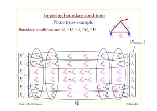
0D D D= = =Boundary conditions are:
Dept. of CE, GCE Kannur Dr.RajeshKN
1 2 8
0D D DBoundary conditions are:](https://image.slidesharecdn.com/module3-directstiffness-rajeshsir-140806045935-phpapp02/85/Module3-direct-stiffness-rajesh-sir-84-320.jpg)
![0.677 -0.177 -0.500 0.000 -0.177⎡ ⎤
⎢ ⎥
Reduced stiffness matrix
[ ]
-0.177 0.677 0.000 0.000 0.177
-0.500 0.000 0.677 0.177 0.000FFS =
⎢ ⎥
⎢ ⎥
⎢ ⎥
⎢ ⎥
[ ]
0.000 0.000 0.177 0.677 0.000
-0.177 0.177 0.000 0.000 0.677
⎢ ⎥
⎢ ⎥
⎢ ⎥⎣ ⎦⎣ ⎦
Dept. of CE, GCE Kannur Dr.RajeshKN
85](https://image.slidesharecdn.com/module3-directstiffness-rajeshsir-140806045935-phpapp02/85/Module3-direct-stiffness-rajesh-sir-85-320.jpg)
![5⎧ ⎫
⎪ ⎪
{ }
0
0FCA
⎪ ⎪
⎪ ⎪⎪ ⎪
= ⎨ ⎬
⎪ ⎪
In this problem, the reduced load vector
(in global coords) can be directly written as
0
0
⎪ ⎪
⎪ ⎪
⎪ ⎪⎩ ⎭
{ } [ ] { }
1
F FF FCD S A
−
=
24.144⎧ ⎫
⎪ ⎪
4.829 1.000 3.829 -1.000 1.000 5⎡ ⎤ ⎧ ⎫
⎢ ⎥ ⎪ ⎪ 5.000
19.144
⎪ ⎪
⎪ ⎪⎪ ⎪
⎨ ⎬
⎪
=
⎪
1.000 1.793 0.793 -0.207 -0.207
3.829 0.793 4.622 -1.207 0.793=
0
0
⎢ ⎥ ⎪ ⎪
⎢ ⎥ ⎪ ⎪⎪ ⎪
⎢ ⎥ ⎨ ⎬
⎢ ⎥ ⎪ ⎪ -5.000
5.000
⎪
⎪
⎪
⎪
⎪
⎪⎩ ⎭
-1.000 -0.207 -1.207 1.793 -0.207 0
1.000 -0.207 0.793 -0.207 1.793 0
⎢ ⎥ ⎪ ⎪
⎢ ⎥ ⎪ ⎪
⎢ ⎥ ⎪ ⎪⎣ ⎦ ⎩ ⎭
Dept. of CE, GCE Kannur Dr.RajeshKN
⎣ ⎦ ⎩ ⎭](https://image.slidesharecdn.com/module3-directstiffness-rajeshsir-140806045935-phpapp02/85/Module3-direct-stiffness-rajesh-sir-86-320.jpg)
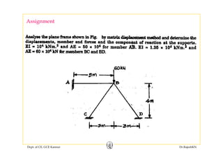

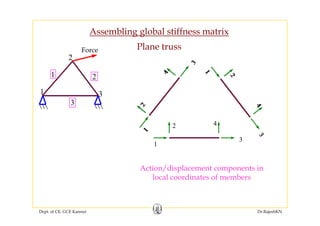
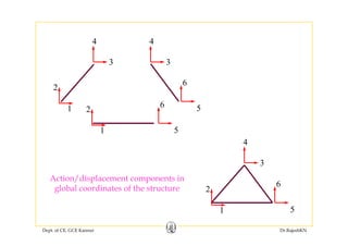
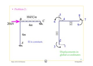
This document discusses the direct stiffness method for structural analysis. It begins by introducing the direct stiffness method and its key aspects, including using member stiffness matrices to express actions and displacements at both ends of each member. It then provides examples of applying the direct stiffness method to analyze a plane truss member and plane frame member. This involves deriving the member stiffness matrices in local coordinates, and transforming displacement, load, and stiffness matrices between local and global coordinate systems using rotation matrices.