Download as PDF, PPTX

![Dept. of CE, GCE Kannur Dr.RajeshKN
8
1 11 1 12 2 13 3 1
2 21 1 22 2 23 3 2
1 1 2 2 3 3
...
...
............................................................
...
n n
n n
n n n n nn n
A S D S D S D S D
A S D S D S D S D
A S D S D S D S D
= + + + +
= + + + +
= + + + +
1 11 12 1 1
2 21 22 2 2
1 2
11
...
...
... ... ... ... ......
...
n
n
n n nn nn
n n nn
A S S S D
A S S S D
S S S DA
× ××
⎧ ⎫ ⎧ ⎫⎧ ⎫
⎪ ⎪ ⎪ ⎪⎪ ⎪
⎪ ⎪ ⎪ ⎪⎪ ⎪
=⎨ ⎬ ⎨ ⎬⎨ ⎬
⎪ ⎪ ⎪ ⎪⎪ ⎪
⎪ ⎪ ⎪ ⎪⎪ ⎪⎩ ⎭⎩ ⎭⎩ ⎭
A = SD
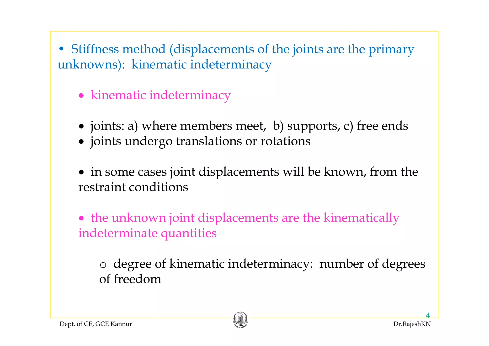
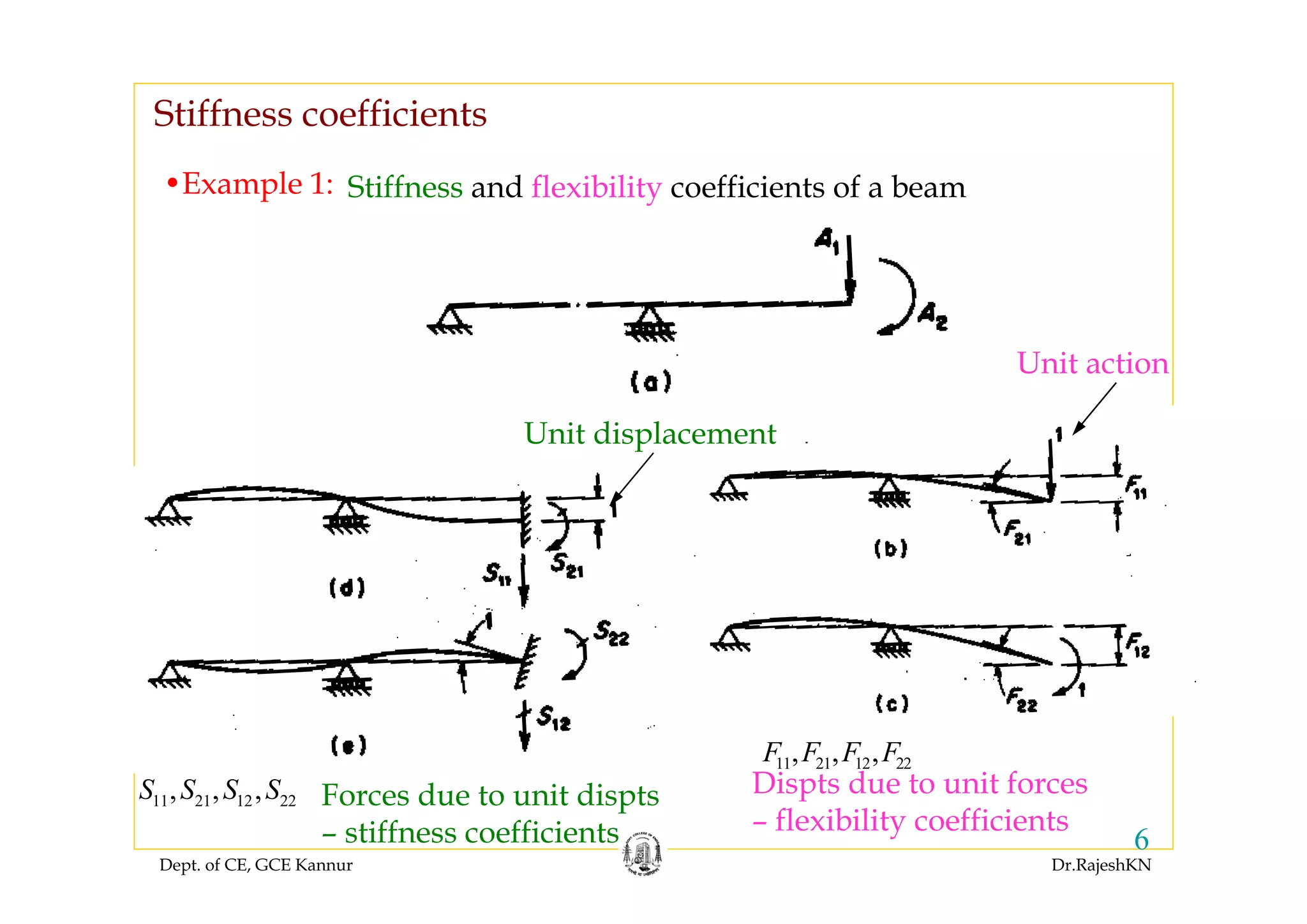
•Action matrix, Stiffness matrix, Displacement matrix
•Stiffness coefficient ijS
{ } [ ] { } [ ] [ ]
1 1
A F D S F
− −
= ⇒ =
oIn matrix form,
{ } [ ]{ }A S D=
[ ] [ ]
1
F S
−
=
Stiffness matrix](https://image.slidesharecdn.com/module2-stiffness-rajeshsir-140806045716-phpapp01/75/Module2-stiffness-rajesh-sir-8-2048.jpg)
![Dept. of CE, GCE Kannur Dr.RajeshKN
12
Stiffnesses of prismatic members
Stiffness coefficients of a structure are calculated from the
contributions of individual members
Hence it is worthwhile to construct member stiffness
matrices
[ ] [ ] 1
Mi MiS F
−
=](https://image.slidesharecdn.com/module2-stiffness-rajeshsir-140806045716-phpapp01/75/Module2-stiffness-rajesh-sir-12-2048.jpg)
![Dept. of CE, GCE Kannur Dr.RajeshKN
13
Member stiffness matrix for prismatic beam member with
rotations at the ends as degrees of freedom
[ ]
2 12
1 2
Mi
EI
S
L
⎡ ⎤
= ⎢ ⎥
⎣ ⎦
[ ] [ ]
1
1
1 2 13 6
1 26
6 3
Mi Mi
L L
LEI EI
S F
L L EI
EI EI
−
−
−
−⎡ ⎤
⎢ ⎥ −⎛ ⎞⎡ ⎤
= = =⎢ ⎥ ⎜ ⎟⎢ ⎥− −⎣ ⎦⎝ ⎠⎢ ⎥
⎢ ⎥⎣ ⎦
2 1 2 16 2
1 2 1 2(3)
EI EI
L L
⎡ ⎤ ⎡ ⎤
= =⎢ ⎥ ⎢ ⎥
⎣ ⎦ ⎣ ⎦
Verification:
B
A
1](https://image.slidesharecdn.com/module2-stiffness-rajeshsir-140806045716-phpapp01/75/Module2-stiffness-rajesh-sir-13-2048.jpg)
![Dept. of CE, GCE Kannur Dr.RajeshKN
14
[ ] 11 12
21 22
3 2
2
12 6
6 4
M M
Mi
M M
S S
S
S S
EI EI
L L
EI EI
L L
⎡ ⎤
= ⎢ ⎥
⎣ ⎦
⎡ ⎤
−⎢ ⎥
= ⎢ ⎥
⎢ ⎥−
⎢ ⎥⎣ ⎦
Member stiffness matrix for prismatic beam member with
deflection and rotation at one end as degrees of freedom](https://image.slidesharecdn.com/module2-stiffness-rajeshsir-140806045716-phpapp01/75/Module2-stiffness-rajesh-sir-14-2048.jpg)
![Dept. of CE, GCE Kannur Dr.RajeshKN
[ ] [ ]
13 2
1
2
1
2
2 33 2
6 3 6
2
Mi Mi
L L
L LLEI EI
S F
EI LL L
EI EI
−
−
−
⎡ ⎤
⎢ ⎥ ⎛ ⎞⎡ ⎤
= = =⎢ ⎥ ⎜ ⎟⎢ ⎥⎜ ⎟⎢ ⎥ ⎣ ⎦⎝ ⎠
⎢ ⎥⎣ ⎦
( )
2
2
3
2
2
6 36
3
12 6
6 423
EI EI
L L
EI EI
L
LEI
L LL L
L
−⎡ ⎤
= =⎢ ⎥−⎣
⎡ ⎤
−⎢ ⎥
⎢ ⎥
⎢
⎢
⎦ ⎥−
⎥⎣ ⎦
Verification:
[ ]Mi
EA
S
L
=
•Truss member](https://image.slidesharecdn.com/module2-stiffness-rajeshsir-140806045716-phpapp01/75/Module2-stiffness-rajesh-sir-15-2048.jpg)
![Dept. of CE, GCE Kannur Dr.RajeshKN
16
•Plane frame member
[ ]
11 12 13
21 22 23
31 32 33
3 2
2
0 0
12 6
0
6 4
0
M M M
Mi M M M
M M M
S S S
S S S S
S S S
EA
L
EI EI
L L
EI EI
L L
⎡ ⎤
⎢ ⎥=
⎢ ⎥
⎢ ⎥⎣ ⎦
⎡ ⎤
⎢ ⎥
⎢ ⎥
⎢ ⎥= −
⎢ ⎥
⎢ ⎥
⎢ ⎥−
⎣ ⎦](https://image.slidesharecdn.com/module2-stiffness-rajeshsir-140806045716-phpapp01/75/Module2-stiffness-rajesh-sir-16-2048.jpg)
![Dept. of CE, GCE Kannur Dr.RajeshKN
17
•Grid member
[ ]
3 2
2
12 6
0
0 0
6 4
0
Mi
EI EI
L L
GJ
S
L
EI EI
L L
⎡ ⎤
−⎢ ⎥
⎢ ⎥
⎢ ⎥=
⎢ ⎥
⎢ ⎥
⎢ ⎥−
⎣ ⎦](https://image.slidesharecdn.com/module2-stiffness-rajeshsir-140806045716-phpapp01/75/Module2-stiffness-rajesh-sir-17-2048.jpg)
![Dept. of CE, GCE Kannur Dr.RajeshKN
18
•Space frame member
[ ]
3 2
3 2
2
2
0 0 0 0 0
12 6
0 0 0 0
12 6
0 0 0 0
0 0 0 0 0
6 4
0 0 0 0
6 4
0 0 0 0
Z Z
Y Y
Mi
Y Y
Z Z
EA
L
EI EI
L L
EI EI
L LS
GJ
L
EI EI
L L
EI EI
L L
⎡ ⎤
⎢ ⎥
⎢ ⎥
⎢ ⎥−
⎢ ⎥
⎢ ⎥
⎢ ⎥
⎢ ⎥=
⎢ ⎥
⎢ ⎥
⎢ ⎥
⎢ ⎥
⎢ ⎥
⎢ ⎥
⎢ ⎥−
⎢ ⎥⎣ ⎦](https://image.slidesharecdn.com/module2-stiffness-rajeshsir-140806045716-phpapp01/75/Module2-stiffness-rajesh-sir-18-2048.jpg)
![Dept. of CE, GCE Kannur Dr.RajeshKN
19
(Explanation using principle of complimentary virtual work)
Formalization of the Stiffness method
{ } [ ]{ }Mi Mi MiA S D=
Here{ }MiD contains relative displacements of the k end with respect
to j end of the i-th member
If there are m members in the structure,
{ }
{ }
{ }
{ }
{ }
[ ] [ ] [ ] [ ] [ ]
[ ] [ ] [ ] [ ] [ ]
[ ] [ ] [ ] [ ] [ ]
[ ] [ ] [ ] [ ] [ ]
[ ] [ ] [ ] [ ] [ ]
{ }
{ }
{ }
{ }
{ }
11 1
22 2
33 3
0 0 0 0
0 0 0 0
0 0 0 0
0 0 0 0
0 0 0 0
MM M
MM M
MM M
MiMi Mi
MmMm Mm
SA D
SA D
SA D
SA D
SA D
⎧ ⎫ ⎧ ⎫⎡ ⎤
⎪ ⎪ ⎪ ⎪⎢ ⎥
⎪ ⎪ ⎪ ⎪⎢ ⎥
⎪ ⎪ ⎪ ⎪⎢ ⎥
⎪ ⎪ ⎪ ⎪⎢ ⎥
=⎨ ⎬ ⎨ ⎬⎢ ⎥
⎪ ⎪ ⎪ ⎪⎢ ⎥
⎪ ⎪ ⎪ ⎪⎢ ⎥
⎪ ⎪ ⎪ ⎪⎢ ⎥
⎪ ⎪ ⎪ ⎪⎢ ⎥
⎩ ⎭ ⎩ ⎭⎣ ⎦
M M MA = S D](https://image.slidesharecdn.com/module2-stiffness-rajeshsir-140806045716-phpapp01/75/Module2-stiffness-rajesh-sir-19-2048.jpg)
![Dept. of CE, GCE Kannur Dr.RajeshKN
20
{ } [ ]{ }M M MA S D=
[ ]MS is the unassembled stiffness matrix of the entire structure](https://image.slidesharecdn.com/module2-stiffness-rajeshsir-140806045716-phpapp01/75/Module2-stiffness-rajesh-sir-20-2048.jpg)
![Dept. of CE, GCE Kannur Dr.RajeshKN
21
• Relative end-displacements in will be related to a vector of joint
displacements for the whole structure,
{ }MD
{ }JD
• If there are no support displacements specified,
{ }RD will be a null matrix
• Hence, { } [ ]{ } [ ] [ ]
{ }
{ }
F
M MJ J MF MR
R
D
D C D C C
D
⎧ ⎫
= = ⎡ ⎤ ⎨ ⎬⎣ ⎦
⎩ ⎭
{ }JD
{ }FDfree (unknown) joint displacements
{ }RDand restraint displacements
consists of:
{ } [ ]{ }M MJ JD C D=
displacement transformation matrix (compatibility matrix)[ ]MJC](https://image.slidesharecdn.com/module2-stiffness-rajeshsir-140806045716-phpapp01/75/Module2-stiffness-rajesh-sir-21-2048.jpg)
![Dept. of CE, GCE Kannur Dr.RajeshKN
22
• Elements in displacement transformation matrix
(compatibility matrix) [ ]MJC are found from compatibility conditions.
•Each column in the submatrix consists of member
displacements caused by a unit value of a support displacement
applied to the restrained structure.
[ ]MRC
[ ]MFC• Each column in the submatrix consists of member
displacements caused by a unit value of an unknown displacement
applied to the restrained structure.
{ }MDrelate to respectively
[ ]MFC
[ ]MRC
and
{ }FD
{ }RD
and](https://image.slidesharecdn.com/module2-stiffness-rajeshsir-140806045716-phpapp01/75/Module2-stiffness-rajesh-sir-22-2048.jpg)
![Dept. of CE, GCE Kannur Dr.RajeshKN
23
{ }MDδ
{ } [ ]{ } [ ] [ ]
{ }
{ }
F
M MJ J MF MR
R
D
D C D C C
D
δ
δ δ
δ
⎧ ⎫
= = ⎡ ⎤ ⎨ ⎬⎣ ⎦
⎩ ⎭
• Suppose an arbitrary set of virtual displacements
is applied on the structure.
{ } { } { } { }
T T T F
J J F R
R
D
W A D A A
D
δ
δ δ δ
δ
⎧ ⎫⎡ ⎤= = ⎨ ⎬⎣ ⎦ ⎩ ⎭
{ }JDδ• External virtual work produced by the virtual displacements
{ }JAand real loads is](https://image.slidesharecdn.com/module2-stiffness-rajeshsir-140806045716-phpapp01/75/Module2-stiffness-rajesh-sir-23-2048.jpg)
![Dept. of CE, GCE Kannur Dr.RajeshKN
24
{ } { }
T
M MU A Dδ δ=
• Internal virtual work produced by the virtual (relative) end
displacements { }MDδ { }MAand actual member end actions is
{ } { } { } { }
T T
J J M MA D A Dδ δ=
• Equating the above two (principle of virtual work),
{ } [ ]{ }M MJ JD C D= { } [ ]{ }M M MA S D=But and
{ } [ ]{ }M MJ JD C Dδ δ=Also,
{ } { } { } [ ] [ ] [ ]{ }
TT T T
J J J MJ M MJ JA D D C S C Dδ δ=Hence,
{ } [ ]{ }J J JA S D=](https://image.slidesharecdn.com/module2-stiffness-rajeshsir-140806045716-phpapp01/75/Module2-stiffness-rajesh-sir-24-2048.jpg)
![Dept. of CE, GCE Kannur Dr.RajeshKN
25
[ ] [ ] [ ][ ]T
J MJ M MJS C S C=Where, , the assembled stiffness matrix for the
entire structure.
• It is useful to partition into submatrices pertaining to free
(unknown) joint displacements
[ ]JS
{ }FD { }RDand restraint displacements
{ } [ ]{ }
{ }
{ }
[ ] [ ]
[ ] [ ]
{ }
{ }
FF FRF F
J J J
RF RRR R
S SA D
A S D
S SA D
⎧ ⎫ ⎧ ⎫⎡ ⎤
= ⇒ =⎨ ⎬ ⎨ ⎬⎢ ⎥
⎩ ⎭ ⎩ ⎭⎣ ⎦
[ ] [ ] [ ][ ]T
FF MF M MFS C S C= [ ] [ ] [ ][ ]T
FR MF M MRS C S C=
[ ] [ ] [ ][ ]T
RF MR M MFS C S C= [ ] [ ] [ ][ ]T
RR MR M MRS C S C=
Where,](https://image.slidesharecdn.com/module2-stiffness-rajeshsir-140806045716-phpapp01/75/Module2-stiffness-rajesh-sir-25-2048.jpg)
![Dept. of CE, GCE Kannur Dr.RajeshKN
26
{ } [ ]{ } [ ]{ }F FF F FR RA S D S D= + { } [ ]{ } [ ]{ }R RF F RR RA S D S D= +
{ } [ ] { } [ ]{ }
1
F FF F FR RD S A S D
−
⇒ = −⎡ ⎤⎣ ⎦
{ } { } [ ]{ } [ ]{ }R RC RF F RR RA A S D S D= − + +
• Support reactions
{ }RCA
represents combined joint loads (actual and equivalent) applied
directly to the supports.
If actual or equivalent joint loads are applied directly to the supports,
Joint displacements](https://image.slidesharecdn.com/module2-stiffness-rajeshsir-140806045716-phpapp01/75/Module2-stiffness-rajesh-sir-26-2048.jpg)
![Dept. of CE, GCE Kannur Dr.RajeshKN
27
{ } { } [ ] [ ]{ } [ ]{ }( )M ML M MF F MR RA A S C D C D= + +
• Member end actions are obtained adding member end actions
calculated as above and initial fixed-end actions
{ } { } [ ][ ]{ }M ML M MJ JA A S C D= +i.e.,
{ }MLAwhere represents fixed end actions](https://image.slidesharecdn.com/module2-stiffness-rajeshsir-140806045716-phpapp01/75/Module2-stiffness-rajesh-sir-27-2048.jpg)
![Dept. of CE, GCE Kannur Dr.RajeshKN
28
Important formulae:
Joint displacements:
Member end actions:
Support reactions:
{ } [ ] { } [ ]{ }
1
F FF F FR RD S A S D
−
= ⎡ − ⎤⎣ ⎦
{ } { } [ ]{ } [ ]{ }R RC RF F RR RA A S D S D= − + +
{ } { } [ ] [ ]{ } [ ]{ }( )M ML M MF F MR RA A S C D C D= + +](https://image.slidesharecdn.com/module2-stiffness-rajeshsir-140806045716-phpapp01/75/Module2-stiffness-rajesh-sir-28-2048.jpg)
![Dept. of CE, GCE Kannur Dr.RajeshKN
29
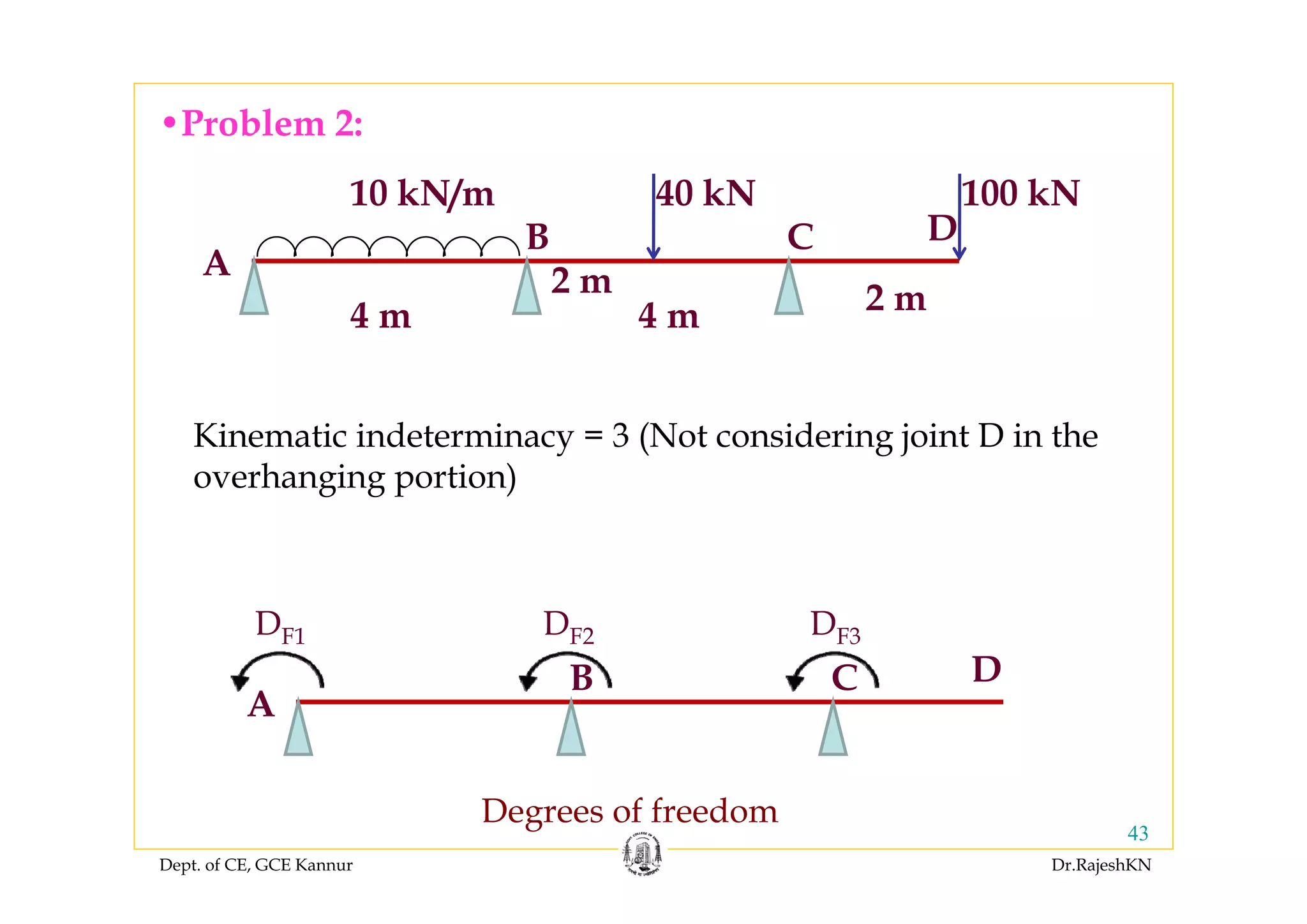
•Problem 1
[ ]
4 2 0 0
2 4 0 02
0 0 2 1
0 0 1 2
M
EI
S
L
⎡ ⎤
⎢ ⎥
⎢ ⎥=
⎢ ⎥
⎢ ⎥
⎣ ⎦
Unassembled stiffness matrix
[ ]
2 12
1 2
Mi
EI
S
L
⎡ ⎤
= ⎢ ⎥
⎣ ⎦
Member stiffness matrix of beam member
Kinematic indeterminacy = 2](https://image.slidesharecdn.com/module2-stiffness-rajeshsir-140806045716-phpapp01/75/Module2-stiffness-rajesh-sir-29-2048.jpg)
![Dept. of CE, GCE Kannur Dr.RajeshKN
Joint displacements
Free (unknown) joint displacements { }FD { }RDRestraint displacements
•Each column in the submatrix consists of member
displacements caused by a unit value of an unknown displacement
applied to the restrained structure.
[ ]MFC
•Each column in the submatrix consists of member
displacements caused by a unit value of a support displacement
applied to the restrained structure.
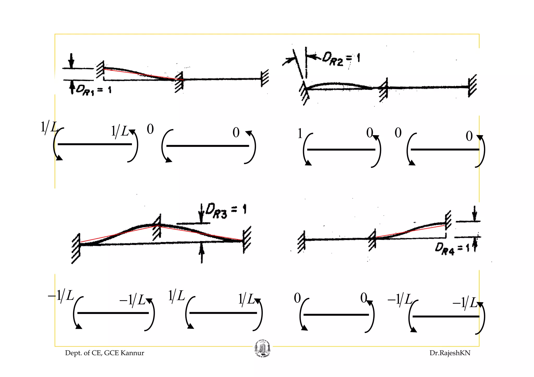
[ ]MRC](https://image.slidesharecdn.com/module2-stiffness-rajeshsir-140806045716-phpapp01/75/Module2-stiffness-rajesh-sir-32-2048.jpg)
![Dept. of CE, GCE Kannur Dr.RajeshKN
0 1 1 0
0 0 0 1
[ ]
0 0
1 0
1 0
0 1
M FC
⎡ ⎤
⎢ ⎥
⎢ ⎥=
⎢ ⎥
⎢ ⎥
⎣ ⎦
DF1 DF2
=1 =1](https://image.slidesharecdn.com/module2-stiffness-rajeshsir-140806045716-phpapp01/75/Module2-stiffness-rajesh-sir-33-2048.jpg)
![Dept. of CE, GCE Kannur Dr.RajeshKN
35
[ ] [ ] [ ]MJ MF MRC C C= ⎡ ⎤⎣ ⎦
0 0 1 1 0
0 1 0 1 01
0 0 0 1 1
0 0 0 1 1
L
L
LL
L
−⎡ ⎤
⎢ ⎥
−⎢ ⎥=
⎢ ⎥−
⎢ ⎥
−⎣ ⎦
[ ]
1 1 1 0
1 0 1 0
0 0 1 1
0 0 1 1
MR
L L
L L
C
L L
L L
−⎡ ⎤
⎢ ⎥−
⎢ ⎥=
−⎢ ⎥
⎢ ⎥
−⎣ ⎦
DR1 DR2 DR3 DR4
=1 =1 =1 =1
DR1 DR2 DR3 DR4
=1 =1 =1 =1
DF1 DF2
=1 =1](https://image.slidesharecdn.com/module2-stiffness-rajeshsir-140806045716-phpapp01/75/Module2-stiffness-rajesh-sir-35-2048.jpg)
![Dept. of CE, GCE Kannur Dr.RajeshKN
36
{ } [ ] { } [ ]{ }
1
F FF F FR RD S A S D
−
= −⎡ ⎤⎣ ⎦
{ } [ ] { }
1
F FF FD S A
−
∴ =
Joint displacements
[ ] [ ] [ ][ ]T
FF MF M MFS C S C=
4 2 0 0 0 0
0 1 1 0 2 4 0 0 1 02
0 0 0 1 0 0 2 1 1 0
0 0 1 2 0 1
EI
L
⎡ ⎤ ⎡ ⎤
⎢ ⎥ ⎢ ⎥
⎡ ⎤ ⎢ ⎥ ⎢ ⎥= ⎢ ⎥ ⎢ ⎥ ⎢ ⎥⎣ ⎦
⎢ ⎥ ⎢ ⎥
⎣ ⎦ ⎣ ⎦
6 12
1 2
EI
L
⎡ ⎤
= ⎢ ⎥
⎣ ⎦
is a null matrix, since there are no support
displacements
{ }RD](https://image.slidesharecdn.com/module2-stiffness-rajeshsir-140806045716-phpapp01/75/Module2-stiffness-rajesh-sir-36-2048.jpg)
![Dept. of CE, GCE Kannur Dr.RajeshKN
{ }
1
6 1 12
1 2 29
F
EI PL
D
L
−
⎛ ⎞⎡ ⎤ ⎧ ⎫
= ⎨ ⎬⎜ ⎟⎢ ⎥
⎣ ⎦ ⎩ ⎭⎝ ⎠
Free (unknown) joint displacements
2 2
01
.
11 818 11
0
11
PL
E EII
PL⎧ ⎫ ⎧
= =
⎫
⎨⎨ ⎬
⎭ ⎩⎩
⎬
⎭
2
3
6 2 3 32
0 0 3 3
L L L LEI
L L L
⎡ ⎤− −
= ⎢ ⎥
−⎣ ⎦
[ ] [ ] [ ][ ]T
FR MF M MRS C S C=
4 2 0 0 1 1 0
0 1 1 0 2 4 0 0 1 0 1 02 1
0 0 0 1 0 0 2 1 0 0 1 1
0 0 1 2 0 0 1 1
L
EI
L L
−⎡ ⎤ ⎡ ⎤
⎢ ⎥ ⎢ ⎥−⎡ ⎤ ⎢ ⎥ ⎢ ⎥= ⎢ ⎥ −⎢ ⎥ ⎢ ⎥⎣ ⎦
⎢ ⎥ ⎢ ⎥
−⎣ ⎦ ⎣ ⎦](https://image.slidesharecdn.com/module2-stiffness-rajeshsir-140806045716-phpapp01/75/Module2-stiffness-rajesh-sir-37-2048.jpg)
![Dept. of CE, GCE Kannur Dr.RajeshKN
{ } { } [ ]{ } [ ]{ }R RC RF F RR RA A S D S D= − + +
is a null matrix.{ }RD
Support reactions
[ ] [ ] [ ][ ]T
RF MR M MFS C S C=
2
6 0
2 02
3 3
3 3
LEI
L
⎡ ⎤
⎢ ⎥
⎢ ⎥=
−⎢ ⎥
⎢ ⎥
− −⎣ ⎦
1 1 0 4 2 0 0 0 0
1 0 1 0 2 4 0 0 1 01 2
0 0 1 1 0 0 2 1 1 0
0 0 1 1 0 0 1 2 0 1
T
L
EI
L L
−⎡ ⎤ ⎡ ⎤ ⎡ ⎤
⎢ ⎥ ⎢ ⎥ ⎢ ⎥−
⎢ ⎥ ⎢ ⎥ ⎢ ⎥=
−⎢ ⎥ ⎢ ⎥ ⎢ ⎥
⎢ ⎥ ⎢ ⎥ ⎢ ⎥
−⎣ ⎦ ⎣ ⎦ ⎣ ⎦
{ } { } [ ]{ }R RC RF FA A S D∴ = − +](https://image.slidesharecdn.com/module2-stiffness-rajeshsir-140806045716-phpapp01/75/Module2-stiffness-rajesh-sir-38-2048.jpg)
![Dept. of CE, GCE Kannur Dr.RajeshKN
[ ] [ ] [ ][ ]T
RR MR M MRS C S C=
1 1 0 4 2 0 0 1 1 0
1 0 1 0 2 4 0 0 1 0 1 01 2 1
0 0 1 1 0 0 2 1 0 0 1 1
0 0 1 1 0 0 1 2 0 0 1 1
T
L L
EI
L L L
− −⎡ ⎤ ⎡ ⎤ ⎡ ⎤
⎢ ⎥ ⎢ ⎥ ⎢ ⎥− −
⎢ ⎥ ⎢ ⎥ ⎢ ⎥=
− −⎢ ⎥ ⎢ ⎥ ⎢ ⎥
⎢ ⎥ ⎢ ⎥ ⎢ ⎥
− −⎣ ⎦ ⎣ ⎦ ⎣ ⎦
3
12 6 12 0
6 4 6 02
12 6 18 6
0 0 6 6
L
L L LEI
LL
−⎡ ⎤
⎢ ⎥−
⎢ ⎥=
− − −⎢ ⎥
⎢ ⎥
−⎣ ⎦](https://image.slidesharecdn.com/module2-stiffness-rajeshsir-140806045716-phpapp01/75/Module2-stiffness-rajesh-sir-39-2048.jpg)
![Dept. of CE, GCE Kannur Dr.RajeshKN
2
2
2
6 0
2 0 02
3
3 3 118
3
3 3
P
PL
LEI PL
L EI
P
P
−⎧ ⎫
⎡ ⎤⎪ ⎪− ⎢ ⎥⎪ ⎪ ⎧ ⎫⎢ ⎥= − +⎨ ⎬ ⎨ ⎬
−⎢ ⎥ ⎩ ⎭⎪ ⎪− ⎢ ⎥⎪ ⎪ − −⎣ ⎦−⎩ ⎭
2
2
0
2 2
0 0
02
3 3
318 33 3
3
3
P P
PL PL
PL EI P
EI L
P P
P
P P
⎧ ⎫
−⎧ ⎫ ⎧ ⎫ ⎪ ⎪⎧ ⎫⎪ ⎪ ⎪ ⎪ ⎪ ⎪− ⎪ ⎪⎪ ⎪ ⎪ ⎪⎪ ⎪ ⎪ ⎪
= − + = +⎨ ⎬ ⎨ ⎬ ⎨ ⎬ ⎨ ⎬
⎪ ⎪ ⎪ ⎪ ⎪ ⎪ ⎪ ⎪−
⎪ ⎪ ⎪ ⎪ ⎪ ⎪ ⎪ ⎪−⎩ ⎭− −⎩ ⎭ ⎩ ⎭ ⎪ ⎪
⎩ ⎭
{ } { } [ ]{ }R RC RF FA A S D∴ = − +
2
3
10
3
2
3
P
PL
P
P
⎧ ⎫
⎪ ⎪
⎪ ⎪
⎪ ⎪⎪ ⎪
⎨ ⎬
⎪ ⎪
⎪ ⎪
⎪ ⎪
⎪ ⎪⎩ ⎭
=](https://image.slidesharecdn.com/module2-stiffness-rajeshsir-140806045716-phpapp01/75/Module2-stiffness-rajesh-sir-40-2048.jpg)
![Dept. of CE, GCE Kannur Dr.RajeshKN
41
{ } { } [ ] [ ]{ } [ ]{ }( )M ML M MF F MR RA A S C D C D= + +
{ }
2
3 4 2 0 0 0 0
3 2 4 0 0 1 0 02
2 0 0 2 1 1 0 19 18
2 0 0 1 2 0 1
M
PL EI PL
A
L EI
⎧ ⎫ ⎡ ⎤ ⎡ ⎤
⎪ ⎪ ⎢ ⎥ ⎢ ⎥− ⎧ ⎫⎪ ⎪ ⎢ ⎥ ⎢ ⎥= +⎨ ⎬ ⎨ ⎬
⎢ ⎥ ⎢ ⎥ ⎩ ⎭⎪ ⎪
⎢ ⎥ ⎢ ⎥⎪ ⎪−⎩ ⎭ ⎣ ⎦ ⎣ ⎦
2
3 4 2 0 0 0
3 2 4 0 0 02
2 0 0 2 1 09 18
2 0 0 1 2 1
PL EI PL
L EI
⎧ ⎫ ⎧ ⎫⎡ ⎤
⎪ ⎪ ⎪ ⎪⎢ ⎥−⎪ ⎪ ⎪ ⎪⎢ ⎥= +⎨ ⎬ ⎨ ⎬
⎢ ⎥⎪ ⎪ ⎪ ⎪
⎢ ⎥⎪ ⎪ ⎪ ⎪−⎩ ⎭ ⎩ ⎭⎣ ⎦
3 0
3 0
2 19 9
2 2
PL PL
⎧ ⎫ ⎧ ⎫
⎪ ⎪ ⎪ ⎪−⎪ ⎪ ⎪ ⎪
= +⎨ ⎬ ⎨ ⎬
⎪ ⎪ ⎪ ⎪
⎪ ⎪ ⎪ ⎪−⎩ ⎭ ⎩ ⎭
1
1
13
0
PL
⎧ ⎫
⎪ ⎪−⎪ ⎪
⎨ ⎬
⎪
⎪
=
⎪
⎪⎩ ⎭
is a null matrix{ }RD
Member end actions
{ } { } [ ][ ]{ }M ML M MF FA A S C D∴ = +](https://image.slidesharecdn.com/module2-stiffness-rajeshsir-140806045716-phpapp01/75/Module2-stiffness-rajesh-sir-41-2048.jpg)
![Dept. of CE, GCE Kannur Dr.RajeshKN
42
3
0 0
0 0 0 2 0 6 4 6 0
1 1 0 0 4 0 6 2 6 02
0 0 0 2 0 0 3 3
1 1 1 1 2 0 0 3 3
0 0 1 1
L L
L L L
L LEI
L L LL
L L
⎡ ⎤
⎢ ⎥ −⎡ ⎤⎢ ⎥
⎢ ⎥−⎢ ⎥
⎢ ⎥= ⎢ ⎥
−⎢ ⎥⎢ ⎥
⎢ ⎥⎢ ⎥− − −⎣ ⎦
⎢ ⎥
− −⎣ ⎦
[ ] [ ]
[ ] [ ]
2 2 2
2 2
3 2
6 6 2 3 3
2 0 0 3 3
6 0 12 6 12 02
2 0 6 4 6 0
3 3 12 6 18 6
3 3 0 0 6 6
FF FR
RF RR
L L L L L L
L L L L
S SL LEI
S SL L L L L
L L L
L L
⎡ ⎤− −
⎢ ⎥
−⎢ ⎥
⎢ ⎥ ⎡ ⎤−
= =⎢ ⎥ ⎢ ⎥
− ⎣ ⎦⎢ ⎥
⎢ ⎥− − − −
⎢ ⎥
− − −⎣ ⎦
[ ] [ ] [ ][ ]T
J MJ M MJS C S C=
0 0
0 0 0 4 2 0 0 0 0 1 1 0
1 1 0 0 2 4 0 0 0 1 0 1 01 2 1
0 0 0 0 0 2 1 0 0 0 1 1
1 1 1 1 0 0 1 2 0 0 0 1 1
0 0 1 1
L L
L L
LEI
L LL L L
L
⎡ ⎤
⎢ ⎥ −⎡ ⎤⎡ ⎤⎢ ⎥ ⎢ ⎥⎢ ⎥ −⎢ ⎥ ⎢ ⎥⎢ ⎥= ⎢ ⎥ ⎢ ⎥−⎢ ⎥⎢ ⎥ ⎢ ⎥⎢ ⎥⎢ ⎥− − −⎣ ⎦ ⎣ ⎦
⎢ ⎥
− −⎣ ⎦
Alternatively, if the entire [SJ] matrix is assembled at a time,](https://image.slidesharecdn.com/module2-stiffness-rajeshsir-140806045716-phpapp01/75/Module2-stiffness-rajesh-sir-42-2048.jpg)
![Dept. of CE, GCE Kannur Dr.RajeshKN
44
[ ]
2 1 0 0
1 2 0 02
0 0 2 14
0 0 1 2
M
EI
S
⎡ ⎤
⎢ ⎥
⎢ ⎥=
⎢ ⎥
⎢ ⎥
⎣ ⎦
Unassembled stiffness matrix
[ ]
2 12
1 24
Mi
EI
S
⎡ ⎤
= ⎢ ⎥
⎣ ⎦
Member stiffness matrix of beam member](https://image.slidesharecdn.com/module2-stiffness-rajeshsir-140806045716-phpapp01/75/Module2-stiffness-rajesh-sir-44-2048.jpg)
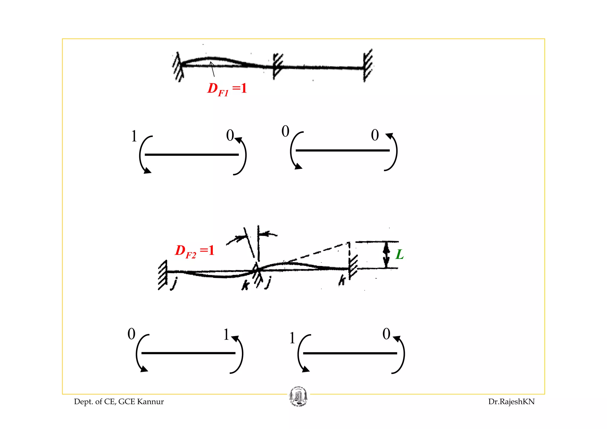
![Dept. of CE, GCE Kannur Dr.RajeshKN
47
[ ]
1 0 0
0 1 0
0 1 0
0 0 1
M FC
⎡ ⎤
⎢ ⎥
⎢ ⎥=
⎢ ⎥
⎢ ⎥
⎣ ⎦
DF1 DF2 DF3
=1 =1 =1
0 0 0 1
DF3 =1](https://image.slidesharecdn.com/module2-stiffness-rajeshsir-140806045716-phpapp01/75/Module2-stiffness-rajesh-sir-47-2048.jpg)
![Dept. of CE, GCE Kannur Dr.RajeshKN
48
{ } [ ] { }
1
F FF FD S A
−
∴ =
Joint displacements
[ ] [ ] [ ][ ]T
FF MF M MFS C S C=
1 0 0 2 1 0 0 1 0 0
0 1 0 1 2 0 0 0 1 02
0 1 0 0 0 2 1 0 1 04
0 0 1 0 0 1 2 0 0 1
T
EI
⎡ ⎤ ⎡ ⎤ ⎡ ⎤
⎢ ⎥ ⎢ ⎥ ⎢ ⎥
⎢ ⎥ ⎢ ⎥ ⎢ ⎥=
⎢ ⎥ ⎢ ⎥ ⎢ ⎥
⎢ ⎥ ⎢ ⎥ ⎢ ⎥
⎣ ⎦ ⎣ ⎦ ⎣ ⎦
1 0.5 0
0.5 2 0.5
0 0.5 1
EI
⎡ ⎤
⎢ ⎥=
⎢ ⎥
⎢ ⎥⎣ ⎦
is a null matrix.{ }RD∴](https://image.slidesharecdn.com/module2-stiffness-rajeshsir-140806045716-phpapp01/75/Module2-stiffness-rajesh-sir-48-2048.jpg)
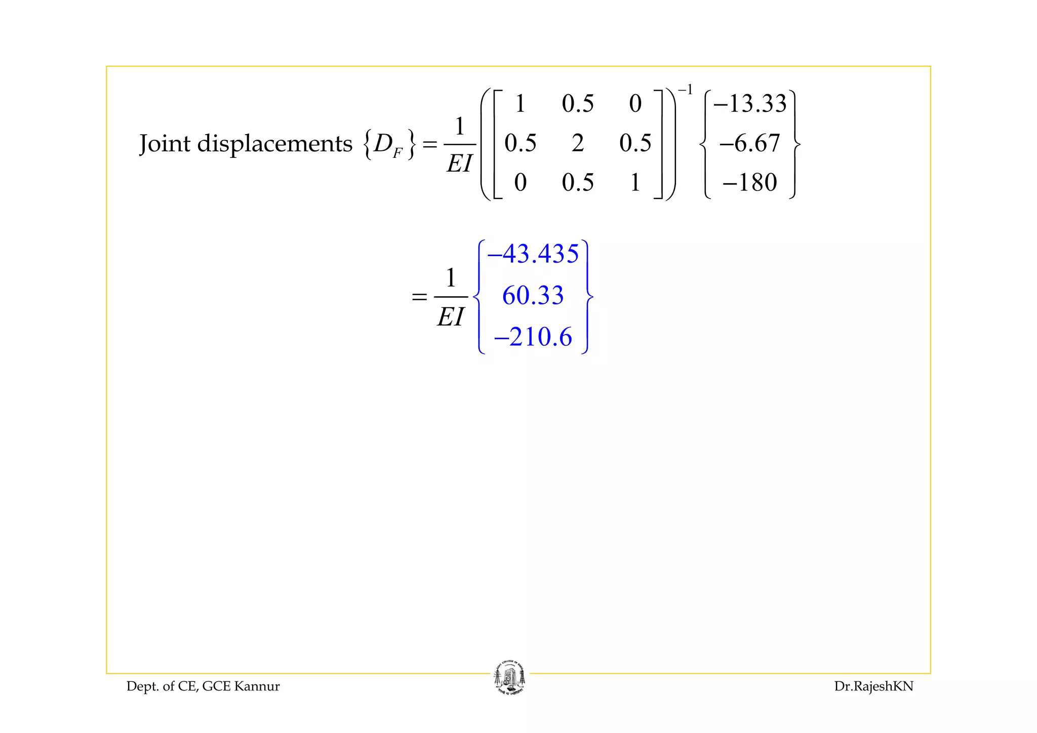
![Dept. of CE, GCE Kannur Dr.RajeshKN
50
{ } { } [ ] [ ]{ } [ ]{ }( )M ML M MF F MR RA A S C D C D= + +
{ }
43.435
60.33
210.6
13.33 2 1 0 0 1 0 0
13.33 1 2 0 0 0 1 02 1
20 0 0 2 1 0 1 04
20 0 0 1 2 0 0 1
M
EI
A
EI
⎧ ⎫ ⎡ ⎤ ⎡ ⎤
⎪ ⎪ ⎢ ⎥ ⎢ ⎥−⎪ ⎪ ⎢ ⎥ ⎢ ⎥= +⎨ ⎬
⎢ ⎥ ⎢ ⎥⎪ ⎪
⎢ ⎥ ⎢ ⎥⎪ ⎪−
−⎧ ⎫
⎪ ⎪
⎨ ⎬
⎪ ⎪−
⎣
⎩
⎭ ⎦ ⎣ ⎦
⎭
⎩
0
25
25
200
kNm
⎧ ⎫
⎪ ⎪
⎪ ⎪
⎨ ⎬
−⎪ ⎪
⎪ ⎪−⎩ ⎭
=
is a null matrix{ }RD
Member end actions
{ } { } [ ][ ]{ }M ML M MF FA A S C D∴ = +](https://image.slidesharecdn.com/module2-stiffness-rajeshsir-140806045716-phpapp01/75/Module2-stiffness-rajesh-sir-50-2048.jpg)
![Dept. of CE, GCE Kannur Dr.RajeshKN
•Problem 3
Analyse the beam. Support B has a downward settlement of 30mm.
EI=5.6×10³ kNm2
[ ]
4 2 0 0 0 0
2 4 0 0 0 0
0 0 2 1 0 02
0 0 1 2 0 06
0 0 0 0 4 2
0 0 0 0 2 4
M
EI
S
⎡ ⎤
⎢ ⎥
⎢ ⎥
⎢ ⎥
= ⎢ ⎥
⎢ ⎥
⎢ ⎥
⎢ ⎥
⎣ ⎦
Unassembled stiffness matrix
[ ]
2 12
1 2Mi
EI
S
L
⎡ ⎤
= ⎢ ⎥
⎣ ⎦
Member stiffness matrix of beam member](https://image.slidesharecdn.com/module2-stiffness-rajeshsir-140806045716-phpapp01/75/Module2-stiffness-rajesh-sir-51-2048.jpg)
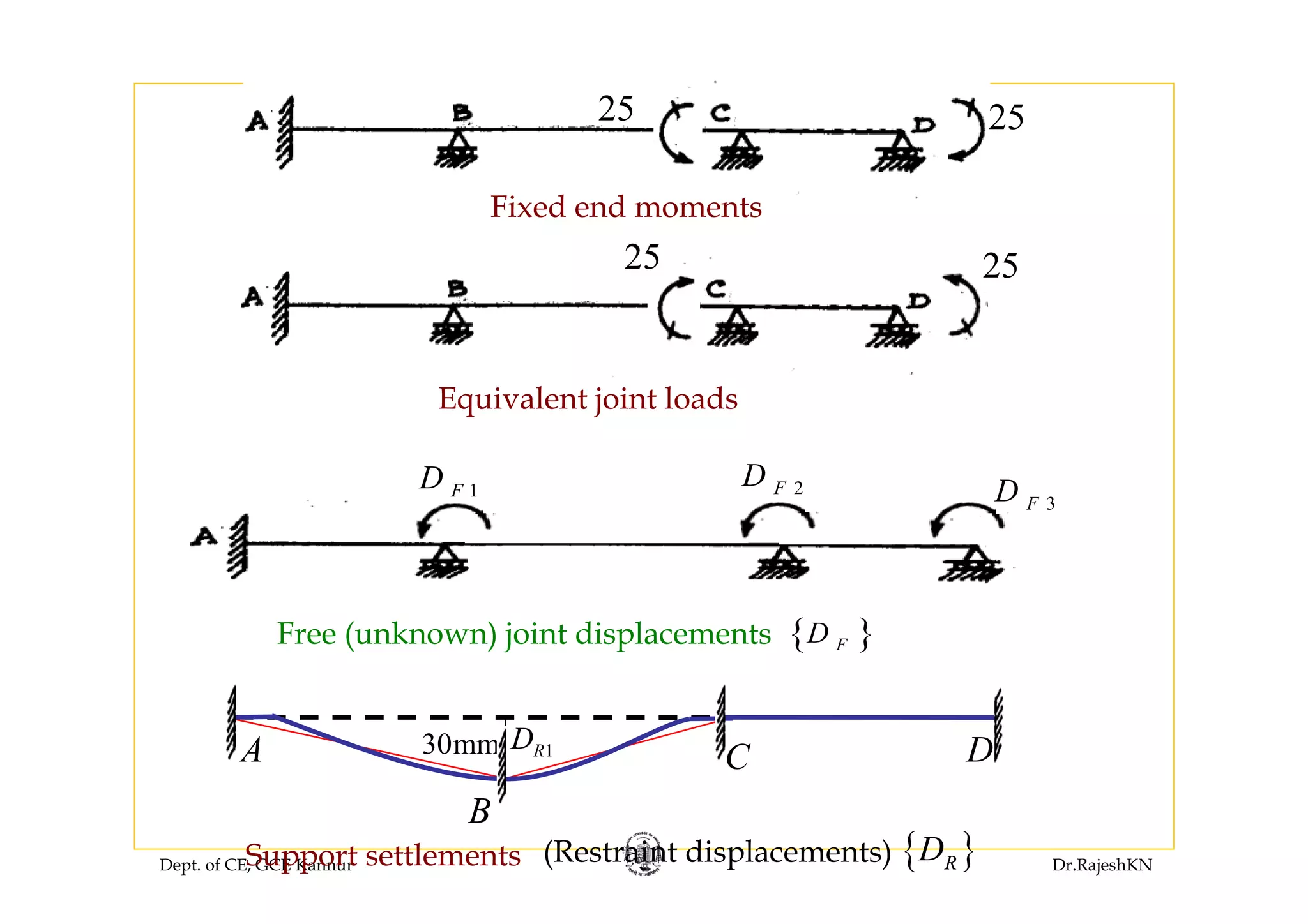
![Dept. of CE, GCE Kannur Dr.RajeshKN
53
BA C D
1 1FD =
0 1 1 0 0 0
and consist of member displacements due to unit
displacements on the restrained structure.
[ ]MFC [ ]MRC](https://image.slidesharecdn.com/module2-stiffness-rajeshsir-140806045716-phpapp01/75/Module2-stiffness-rajesh-sir-53-2048.jpg)
![Dept. of CE, GCE Kannur Dr.RajeshKN
54
[ ] [ ] [ ]MJ MF MRC C C= ⎡ ⎤⎣ ⎦
0 0 0 1 3
1 0 0 1 3
1 0 0 1 6
0 1 0 1 6
0 1 0 0
0 0 1 0
−⎡ ⎤
⎢ ⎥
−⎢ ⎥
⎢ ⎥
= ⎢ ⎥
⎢ ⎥
⎢ ⎥
⎢ ⎥
⎢ ⎥⎣ ⎦
31 2 1
1 1 11
FF F RDD D D
= = ==
A
B
C D1 1RD =
1 3− 1 3− 1 6 1 6 0 0](https://image.slidesharecdn.com/module2-stiffness-rajeshsir-140806045716-phpapp01/75/Module2-stiffness-rajesh-sir-54-2048.jpg)
![Dept. of CE, GCE Kannur Dr.RajeshKN
55
{ } [ ] { } [ ]{ }
1
F FF F FR RD S A S D
−
= −⎡ ⎤⎣ ⎦
Joint displacements
[ ] [ ] [ ][ ]T
FF MF M MFS C S C=
0 0 0 4 2 0 0 0 0 0 0 0
1 0 0 2 4 0 0 0 0 1 0 0
1 0 0 0 0 2 1 0 0 1 0 0
0 1 0 0 0 1 2 0 0 0 1 03
0 1 0 0 0 0 0 4 2 0 1 0
0 0 1 0 0 0 0 2 4 0 0 1
T
EI
⎡ ⎤ ⎡ ⎤ ⎡ ⎤
⎢ ⎥ ⎢ ⎥ ⎢ ⎥
⎢ ⎥ ⎢ ⎥ ⎢ ⎥
⎢ ⎥ ⎢ ⎥ ⎢ ⎥
= ⎢ ⎥ ⎢ ⎥ ⎢ ⎥
⎢ ⎥ ⎢ ⎥ ⎢ ⎥
⎢ ⎥ ⎢ ⎥ ⎢ ⎥
⎢ ⎥ ⎢ ⎥ ⎢ ⎥
⎣ ⎦ ⎣ ⎦ ⎣ ⎦
6 1 0
1 6 2
3
0 2 4
EI
⎡ ⎤
⎢ ⎥=
⎢ ⎥
⎢ ⎥⎣ ⎦](https://image.slidesharecdn.com/module2-stiffness-rajeshsir-140806045716-phpapp01/75/Module2-stiffness-rajesh-sir-55-2048.jpg)
![Dept. of CE, GCE Kannur Dr.RajeshKN
[ ] [ ] [ ][ ]T
FR MF M MRS C S C=
0 0 0 4 2 0 0 0 0 1 3
1 0 0 2 4 0 0 0 0 1 3
1 0 0 0 0 2 1 0 0 1 6
0 1 0 0 0 1 2 0 0 1 63
0 1 0 0 0 0 0 4 2 0
0 0 1 0 0 0 0 2 4 0
T
EI
−⎡ ⎤ ⎡ ⎤ ⎡ ⎤
⎢ ⎥ ⎢ ⎥ ⎢ ⎥−
⎢ ⎥ ⎢ ⎥ ⎢ ⎥
⎢ ⎥ ⎢ ⎥ ⎢ ⎥
= ⎢ ⎥ ⎢ ⎥ ⎢ ⎥
⎢ ⎥ ⎢ ⎥ ⎢ ⎥
⎢ ⎥ ⎢ ⎥ ⎢ ⎥
⎢ ⎥ ⎢ ⎥ ⎢ ⎥
⎣ ⎦ ⎣ ⎦ ⎣ ⎦
3 2
1 2
3
0
EI
−⎧ ⎫
⎪ ⎪
= ⎨ ⎬
⎪ ⎪
⎩ ⎭](https://image.slidesharecdn.com/module2-stiffness-rajeshsir-140806045716-phpapp01/75/Module2-stiffness-rajesh-sir-56-2048.jpg)
![Dept. of CE, GCE Kannur Dr.RajeshKN
{ }
1
6 1 0 0 3 2
1 6 2 25 1 2 0.03
3 3
0 2 4 25 0
EI EI
−
−⎛ ⎞ ⎡ ⎤⎧ ⎫⎡ ⎤ ⎡ ⎤
⎪ ⎪⎜ ⎟ ⎢ ⎥⎢ ⎥ ⎢ ⎥= − − −⎨ ⎬⎜ ⎟ ⎢ ⎥⎢ ⎥ ⎢ ⎥
⎪ ⎪⎜ ⎟ ⎢ ⎥⎢ ⎥ ⎢ ⎥⎩ ⎭⎣ ⎦ ⎣ ⎦⎝ ⎠ ⎣ ⎦
20 4 2 0 0.045
3 5600
4 24 12 25 0.015
116 3
2 12 35 25 0
EI
− ⎡ ⎤⎧ ⎫ ⎧ ⎫⎡ ⎤
⎪ ⎪ ⎪ ⎪⎢ ⎥⎢ ⎥= − − − − −⎨ ⎬ ⎨ ⎬⎢ ⎥⎢ ⎥
⎪ ⎪ ⎪ ⎪⎢ ⎥−⎢ ⎥ ⎩ ⎭ ⎩ ⎭⎣ ⎦ ⎣ ⎦
3
1642
3
108
116 5.6 10
6
0.007583
0.0005
0.007 311
−⎧ ⎫
⎪ ⎪
= =⎨ ⎬
× × ⎪ ⎪
−⎧ ⎫
⎪ ⎪
⎨ ⎬
⎪ ⎪
⎩⎩ ⎭⎭
20 4 2 0 84
3
4 24 12 25 28
116
2 12 35 25 0
EI
− ⎡ ⎤⎧ ⎫ ⎧ ⎫⎡ ⎤
⎪ ⎪ ⎪ ⎪⎢ ⎥⎢ ⎥= − − − − −⎨ ⎬ ⎨ ⎬⎢ ⎥⎢ ⎥
⎪ ⎪ ⎪ ⎪⎢ ⎥−⎢ ⎥ ⎩ ⎭ ⎩ ⎭⎣ ⎦ ⎣ ⎦
{ } [ ] { } [ ]{ }
1
F FF F FR RD S A S D
−
= −⎡ ⎤⎣ ⎦](https://image.slidesharecdn.com/module2-stiffness-rajeshsir-140806045716-phpapp01/75/Module2-stiffness-rajesh-sir-57-2048.jpg)
![Dept. of CE, GCE Kannur Dr.RajeshKN
58
{ } { } [ ]{ } [ ]{ }R RC RF F RR RA A S D S D= − + +
Support reactions
[ ]
4 2 0 0 0 0 0 0 0
2 4 0 0 0 0 1 0 0
0 0 2 1 0 0 1 0 0
1 3 1 3 1 6 1 6 0 0
0 0 1 2 0 0 0 1 03
0 0 0 0 4 2 0 1 0
0 0 0 0 2 4 0 0 1
EI
⎡ ⎤ ⎡ ⎤
⎢ ⎥ ⎢ ⎥
⎢ ⎥ ⎢ ⎥
⎢ ⎥ ⎢ ⎥
= − − ⎢ ⎥ ⎢ ⎥
⎢ ⎥ ⎢ ⎥
⎢ ⎥ ⎢ ⎥
⎢ ⎥ ⎢ ⎥
⎣ ⎦ ⎣ ⎦
[ ] [ ] [ ][ ]T
RF MR M MFS C S C=
[ ]3 2 1 2 0
3
EI
= −](https://image.slidesharecdn.com/module2-stiffness-rajeshsir-140806045716-phpapp01/75/Module2-stiffness-rajesh-sir-58-2048.jpg)
![Dept. of CE, GCE Kannur Dr.RajeshKN
{ } { } [ ] { }
0.007583
0 3 2 1 2 0 0.0005 0.03
3 2
0.0031
R
EI EI
A
−⎧ ⎫
⎪ ⎪ ⎡ ⎤
= − + − + −⎨ ⎬ ⎢ ⎥⎣ ⎦⎪ ⎪
⎩ ⎭
(Support reaction corresponding to DR . i.e., reaction at B)
( )0.0116 0.045 0.0334 62 5
3 3
.3
EI EI
= − = − −=
[ ] [ ] [ ][ ]T
RR MR M MRS C S C=
[ ]
4 2 0 0 0 0 1 3
2 4 0 0 0 0 1 3
0 0 2 1 0 0 1 6
1 3 1 3 1 6 1 6 0 0
0 0 1 2 0 0 1 63
0 0 0 0 4 2 0
0 0 0 0 2 4 0
EI
−⎡ ⎤ ⎡ ⎤
⎢ ⎥ ⎢ ⎥−
⎢ ⎥ ⎢ ⎥
⎢ ⎥ ⎢ ⎥
= − − ⎢ ⎥ ⎢ ⎥
⎢ ⎥ ⎢ ⎥
⎢ ⎥ ⎢ ⎥
⎢ ⎥ ⎢ ⎥
⎣ ⎦ ⎣ ⎦
2
EI⎡ ⎤
= ⎢ ⎥⎣ ⎦](https://image.slidesharecdn.com/module2-stiffness-rajeshsir-140806045716-phpapp01/75/Module2-stiffness-rajesh-sir-59-2048.jpg)
![Dept. of CE, GCE Kannur Dr.RajeshKN
60
{ } { } [ ] [ ]{ } [ ]{ }( )M ML M MF F MR RA A S C D C D= + +
{ } { }
0 4 2 0 0 0 0 0 0 0 1 3
0 2 4 0 0 0 0 1 0 0 1 3
0.007583
0 0 0 2 1 0 0 1 0 0 1 62
0.0005 0.03
0 0 0 1 2 0 0 0 1 0 1 66
0.0031
25 0 0 0 0 4 2 0 1 0 0
25 0 0 0 0 2 4 0 0 1 0
M
EI
A
−⎛⎧ ⎫ ⎡ ⎤ ⎡ ⎤ ⎡ ⎤
⎜⎪ ⎪ ⎢ ⎥ ⎢ ⎥ ⎢ ⎥−⎜⎪ ⎪ ⎢ ⎥ ⎢ ⎥ ⎢ ⎥−⎧ ⎫
⎜⎪ ⎪ ⎢ ⎥ ⎢ ⎥ ⎢ ⎥⎪ ⎪
= + + −⎜⎨ ⎬ ⎨ ⎬⎢ ⎥ ⎢ ⎥ ⎢ ⎥
⎜⎪ ⎪ ⎪ ⎪⎢ ⎥ ⎢ ⎥ ⎢ ⎥
⎩ ⎭⎜⎪ ⎪ ⎢ ⎥ ⎢ ⎥ ⎢ ⎥
⎪ ⎪ ⎢ ⎥ ⎢ ⎥ ⎢ ⎥
−⎩ ⎭ ⎣ ⎦ ⎣ ⎦ ⎣ ⎦⎝
⎞
⎟
⎟
⎟
⎟
⎟
⎟
⎜ ⎟⎜ ⎟
⎠
83.7
55.4
55.4
40.3
40.3
0
⎧ ⎫
⎪ ⎪
⎪ ⎪
−⎪ ⎪
⎨ ⎬
−⎪
⎪
⎪
⎩
=
⎪
⎪
⎪
⎭
Member end actions](https://image.slidesharecdn.com/module2-stiffness-rajeshsir-140806045716-phpapp01/75/Module2-stiffness-rajesh-sir-60-2048.jpg)
![Dept. of CE, GCE Kannur Dr.RajeshKN
61
[ ] [ ]
[ ] [ ]
FF FR
RF RR
S S
S S
⎡ ⎤
= ⎢ ⎥
⎣ ⎦
6 1 0 3 2
1 6 2 1 2
0 2 4 03
3 2 1 2 0 3 2
E I
−⎡ ⎤
⎢ ⎥
⎢ ⎥=
⎢ ⎥
⎢ ⎥
−⎣ ⎦
2 0 0 2
0 1 1 0 0 0 4 0 0 2
0 0 0 1 1 0 2 1 0 1 2
0 0 0 0 0 1 1 2 0 1 23
1 3 1 3 1 6 1 6 0 0 0 4 2 0
0 2 4 0
EI
−⎡ ⎤
⎢ ⎥−⎡ ⎤ ⎢ ⎥
⎢ ⎥ ⎢ ⎥
⎢ ⎥= ⎢ ⎥
⎢ ⎥ ⎢ ⎥
⎢ ⎥ ⎢ ⎥− −⎣ ⎦
⎢ ⎥
⎣ ⎦
[ ] [ ] [ ][ ]T
J MJ M MJS C S C=
4 2 0 0 0 0 0 0 0 1 3
0 1 1 0 0 0 2 4 0 0 0 0 1 0 0 1 3
0 0 0 1 1 0 0 0 2 1 0 0 1 0 0 1 6
0 0 0 0 0 1 0 0 1 2 0 0 0 1 0 1 63
1 3 1 3 1 6 1 6 0 0 0 0 0 0 4 2 0 1 0 0
0 0 0 0 2 4 0 0 1 0
EI
−⎡ ⎤⎡ ⎤
⎢ ⎥⎢ ⎥ −⎡ ⎤ ⎢ ⎥⎢ ⎥
⎢ ⎥ ⎢ ⎥⎢ ⎥
⎢ ⎥= ⎢ ⎥⎢ ⎥
⎢ ⎥ ⎢ ⎥⎢ ⎥
⎢ ⎥ ⎢ ⎥⎢ ⎥− −⎣ ⎦
⎢ ⎥⎢ ⎥
⎢ ⎥⎣ ⎦ ⎣ ⎦
Alternatively, if the entire [SJ] matrix is assembled at a time,](https://image.slidesharecdn.com/module2-stiffness-rajeshsir-140806045716-phpapp01/75/Module2-stiffness-rajesh-sir-61-2048.jpg)
![Dept. of CE, GCE Kannur Dr.RajeshKN
62
[ ] [ ] [ ]MJ MF MRC C C= ⎡ ⎤⎣ ⎦
0 0 0 1 3 1 1 3 0 0
1 0 0 1 3 0 1 3 0 0
1 0 0 0 0 1 6 1 6 0
0 1 0 0 0 1 6 1 6 0
0 1 0 0 0 0 1 3 1 3
0 0 1 0 0 0 1 3 1 3
−⎡ ⎤
⎢ ⎥
−⎢ ⎥
⎢ ⎥−
= ⎢ ⎥
−⎢ ⎥
⎢ ⎥−
⎢ ⎥
−⎢ ⎥⎣ ⎦
[ ] [ ] [ ][ ]T
J MJ M MJS C S C=
0 0 01 3 1 1 3 0 0 4 2 0 0 0 0 0 0 01 3 1 1 3 0 0
1 0 01 3 0 1 3 0 0 2 4 0 0 0 0 1 0 01 3 0 1 3 0 0
1 0 0 0 0 1 6 1 6 0 0 0 2 1 0 0 1 0 0 0 0 1 6 1 6 0
0 1 0 0 0 1 6 1 6 0 0 0 1 2 0 0 0 1 0 0 0 1 6 1 6 03
0 1 0 0 0 0 1 3 1 3 0 0 0 0 4 2 0 1 0 0 0 0 1 3
0 0 1 0 0 0 1 3 1 3 0 0 0 0 2 4 0 0 1
T
EI
− −⎡ ⎤ ⎡ ⎤
⎢ ⎥ ⎢ ⎥− −⎢ ⎥ ⎢ ⎥
⎢ ⎥− −⎢ ⎥
= ⎢ ⎥ ⎢ ⎥
− −⎢ ⎥ ⎢ ⎥
⎢ ⎥ ⎢ ⎥−
⎢ ⎥ ⎢ ⎥
−⎢ ⎥ ⎣ ⎦⎣ ⎦
1 3
0 0 0 1 3 1 3
⎡ ⎤
⎢ ⎥
⎢ ⎥
⎢ ⎥
⎢ ⎥
⎢ ⎥
⎢ ⎥−
⎢ ⎥
−⎢ ⎥⎣ ⎦
Alternatively, if ALL possible support settlements are accounted for,](https://image.slidesharecdn.com/module2-stiffness-rajeshsir-140806045716-phpapp01/75/Module2-stiffness-rajesh-sir-62-2048.jpg)
![Dept. of CE, GCE Kannur Dr.RajeshKN
63
[ ] [ ]
[ ] [ ]
FF FR
RF RR
S S
S S
⎡ ⎤
= ⎢ ⎥
⎣ ⎦
0 1 1 0 0 0
0 0 0 1 1 0 2 0 0 2 4 2 0 0
0 0 0 0 0 1 4 0 0 2 2 2 0 0
1 3 1 3 0 0 0 0 2 1 0 0 0 1 2 1 2 0
1 0 0 0 0 0 1 2 0 0 0 1 2 1 2 03
1 3 1 3 1 6 1 6 0 0 0 4 2 0 0 0 2 2
0 0 1 6 1 6 1 3 1 3 0 2 4 0 0 0 2 2
0 0 0 0 1 3 1 3
EI
⎡ ⎤
⎢ ⎥ −⎡ ⎤⎢ ⎥
⎢ ⎥−⎢ ⎥
⎢ ⎥⎢ ⎥
−⎢ ⎥⎢ ⎥= ⎢ ⎥⎢ ⎥ −⎢ ⎥⎢ ⎥
⎢ ⎥− − −⎢ ⎥
⎢ ⎥⎢ ⎥− − −⎣ ⎦
⎢ ⎥
− −⎣ ⎦
6 1 0 2 2 3 2 1 2 0
1 6 2 0 0 1 2 3 2 2
0 2 4 0 0 0 2 2
2 0 0 4 3 2 4 3 0 0
2 0 0 2 4 2 0 03
3 2 1 2 0 4 3 2 3 2 1 6 0
1 2 3 2 2 0 0 1 6 3 2 4 3
0 2 2 0 0 0 4 3 4 3
EI
− −⎡ ⎤
⎢ ⎥−
⎢ ⎥
−⎢ ⎥
⎢ ⎥
−⎢ ⎥=
⎢ ⎥−
⎢ ⎥
− − − −⎢ ⎥
⎢ ⎥− − −
⎢ ⎥
− − −⎣ ⎦](https://image.slidesharecdn.com/module2-stiffness-rajeshsir-140806045716-phpapp01/75/Module2-stiffness-rajesh-sir-63-2048.jpg)
![Dept. of CE, GCE Kannur Dr.RajeshKN
64
{ } [ ] { } [ ]{ }
1
F FF F FR RD S A S D
−
= −⎡ ⎤⎣ ⎦
1
0
6 1 0 0 2 2 3 2 1 2 0 0
1 6 2 25 0 0 1 2 3 2 2 0.03
3 3
0 2 4 25 0 0 0 2 2 0
0
EI EI
−
⎡ ⎤⎧ ⎫
⎢ ⎥⎪ ⎪− −⎛ ⎞ ⎧ ⎫⎡ ⎤ ⎡ ⎤⎢ ⎥⎪ ⎪⎪ ⎪ ⎪ ⎪⎜ ⎟⎢ ⎥ ⎢ ⎥⎢ ⎥= − − − −⎨ ⎬ ⎨ ⎬⎜ ⎟⎢ ⎥ ⎢ ⎥⎢ ⎥⎪ ⎪ ⎪ ⎪⎜ ⎟ −⎢ ⎥ ⎢ ⎥⎩ ⎭⎣ ⎦ ⎣ ⎦⎝ ⎠ ⎢ ⎥⎪ ⎪
⎢ ⎥⎪ ⎪⎩ ⎭⎣ ⎦
20 4 2 0 0.045
3 5600
4 24 12 25 0.015
116 3
2 12 35 25 0
20 4 2 84
3
4 24 12 3
116
2 12 35 25
EI
EI
− ⎡ ⎤⎧ ⎫ ⎧ ⎫⎡ ⎤
⎪ ⎪ ⎪ ⎪⎢ ⎥⎢ ⎥= − − − − −⎨ ⎬ ⎨ ⎬⎢ ⎥⎢ ⎥
⎪ ⎪ ⎪ ⎪⎢ ⎥−⎢ ⎥ ⎩ ⎭ ⎩ ⎭⎣ ⎦ ⎣ ⎦
− −⎧ ⎫⎡ ⎤
⎪ ⎪⎢ ⎥= − − ⎨ ⎬⎢ ⎥
⎪ ⎪−⎢ ⎥ ⎩ ⎭⎣ ⎦
1642
3
108
116
671
EI
−⎧ ⎫
⎪ ⎪
= ⎨ ⎬
⎪ ⎪
⎩ ⎭
0.007583
0.0005
0.0031
−⎧ ⎫
⎪ ⎪
⎨ ⎬
⎪
⎩
=
⎪
⎭
Joint displacements](https://image.slidesharecdn.com/module2-stiffness-rajeshsir-140806045716-phpapp01/75/Module2-stiffness-rajesh-sir-64-2048.jpg)
![Dept. of CE, GCE Kannur Dr.RajeshKN
65
{ }
0 2 0 0 4 3 2 4 3 0 0 0
0.0075830 2 0 0 2 4 2 0 0 0
0.00050 3 2 1 2 0 4 3 2 3 2 1 6 0 0.03
3 3
0.003150 1 2 3 2 2 0 0 1 6 3 2 4 3 0
50 0 2 2 0 0 0 4 3 4 3 0
R
EI EI
A
−⎧ ⎫ ⎧ ⎫⎡ ⎤ ⎡ ⎤
⎪ ⎪ ⎪ ⎪⎢ ⎥ ⎢ ⎥− −⎧ ⎫⎪ ⎪ ⎪ ⎪⎢ ⎥ ⎢ ⎥⎪ ⎪ ⎪ ⎪ ⎪ ⎪
= − + +− − − − −⎢ ⎥ ⎢ ⎥⎨ ⎬ ⎨ ⎬ ⎨ ⎬
⎢ ⎥ ⎢ ⎥⎪ ⎪ ⎪ ⎪ ⎪ ⎪− − − −⎩ ⎭⎢ ⎥ ⎢ ⎥⎪ ⎪ ⎪ ⎪
⎢ ⎥ ⎢ ⎥− − − −⎪ ⎪ ⎪ ⎪⎩ ⎭ ⎩ ⎭⎣ ⎦ ⎣ ⎦
{ } { } [ ]{ } [ ]{ }R RC RF F RR RA A S D S D= − + +
{ }
0 28.373 74.667
0 28.373 112
0 21.653 84
50 19.973 9.333
46.294
83.627
62.347
79.31
36.5650 13.44 0
RA
−⎧ ⎫ ⎧ ⎫ ⎧ ⎫
⎪ ⎪ ⎪ ⎪ ⎪ ⎪−
⎪ ⎪ ⎪ ⎪ ⎪ ⎪⎪ ⎪ ⎪ ⎪ ⎪ ⎪
= − + + =−⎨ ⎬ ⎨ ⎬ ⎨ ⎬
⎪ ⎪ ⎪ ⎪ ⎪ ⎪−
⎪ ⎪ ⎪ ⎪ ⎪ ⎪
− −⎪ ⎪ ⎪ ⎪ ⎪ ⎪⎩ ⎭ ⎩ ⎭ ⎩
⎧ ⎫
⎪ ⎪
⎪ ⎪⎪ ⎪
−⎨ ⎬
⎪ ⎪
⎪ ⎪
⎪⎩ ⎭⎭ ⎪
Support reactions](https://image.slidesharecdn.com/module2-stiffness-rajeshsir-140806045716-phpapp01/75/Module2-stiffness-rajesh-sir-65-2048.jpg)
![Dept. of CE, GCE Kannur Dr.RajeshKN
66
{ } { } [ ] [ ]{ } [ ]{ }( )M ML M MF F MR RA A S C D C D= + +
{ }
0 4 2 0 0 0 0 0 0 0 1 3 1 1 3 0 0
0 2 4 0 0 0 0 1 0 0 1 3 0 1 3 0 0
0.007583
0 0 0 2 1 0 0 1 0 0 0 0 1 6 1 6 02
0.0005
0 0 0 1 2 0 0 0 1 0 0 0 1 6 1 6 06
0.0031
25 0 0 0 0 4 2 0 1 0 0 0 0 1 3 1 3
25 0 0 0 0 2 4 0 0 1 0 0 0
M
EI
A
−⎧ ⎫ ⎡ ⎤ ⎡ ⎤
⎪ ⎪ ⎢ ⎥ ⎢ ⎥ −
⎪ ⎪ ⎢ ⎥ ⎢ ⎥ −⎧ ⎫
−⎪ ⎪ ⎢ ⎥ ⎢ ⎥ ⎪ ⎪
= + +⎨ ⎬ ⎨ ⎬⎢ ⎥ ⎢ ⎥
−⎪ ⎪ ⎪ ⎪⎢ ⎥ ⎢ ⎥
⎩ ⎭⎪ ⎪ ⎢ ⎥ ⎢ ⎥ −
⎪ ⎪ ⎢ ⎥ ⎢ ⎥
−⎩ ⎭ ⎣ ⎦ ⎣ ⎦
0
0
0.03
0
0
1 3 1 3
⎛ ⎞⎡ ⎤
⎧ ⎫⎜ ⎟⎢ ⎥
⎪ ⎪⎜ ⎟⎢ ⎥
⎪ ⎪⎜ ⎟⎢ ⎥ ⎪ ⎪
−⎜ ⎟⎨ ⎬⎢ ⎥
⎜ ⎟⎪ ⎪⎢ ⎥
⎜ ⎟⎪ ⎪⎢ ⎥
⎜ ⎟⎪ ⎪⎢ ⎥ ⎩ ⎭⎜ ⎟−⎣ ⎦⎝ ⎠
{ }
83.7
55.4
55.4
40.3
40.3
0
MA
⎧ ⎫
⎪ ⎪
⎪ ⎪
−⎪ ⎪
⎨ ⎬
−⎪ ⎪
⎪ ⎪
⎪ ⎪
⎩ ⎭
=
Member end actions](https://image.slidesharecdn.com/module2-stiffness-rajeshsir-140806045716-phpapp01/75/Module2-stiffness-rajesh-sir-66-2048.jpg)
![Dept. of CE, GCE Kannur Dr.RajeshKN
[ ]
2 4 1 4 0 0 0 0
1 4 2 4 0 0 0 0
0 0 6 4.8 3 4.8 0 0
2
0 0 3 4.8 6 4.8 0 0
0 0 0 0 4 8 2 8
0 0 0 0 2 8 4 8
MS EI
⎡ ⎤
⎢ ⎥
⎢ ⎥
⎢ ⎥
= ⎢ ⎥
⎢ ⎥
⎢ ⎥
⎢ ⎥
⎣ ⎦
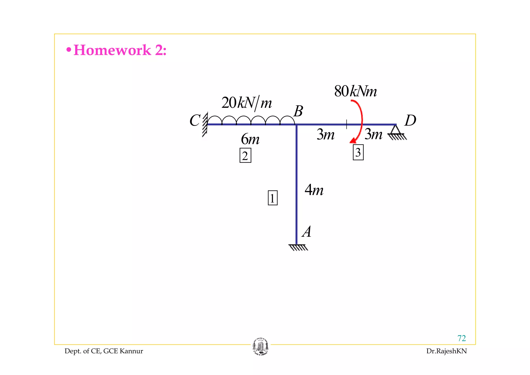
•Problem 4
Unassembled
stiffness matrix
Equivalent joint loads
85.33
42.67
1
2
3](https://image.slidesharecdn.com/module2-stiffness-rajeshsir-140806045716-phpapp01/75/Module2-stiffness-rajesh-sir-67-2048.jpg)
![Dept. of CE, GCE Kannur Dr.RajeshKN
68
• consists of member displacements due to unit displacements on
the restrained structure.
[ ]MFC
1 1FD =
2 1FD =
[ ]
1 0
0 1
0 0
0 1
0 1
0 0
MFC
⎡ ⎤
⎢ ⎥
⎢ ⎥
⎢ ⎥
= ⎢ ⎥
⎢ ⎥
⎢ ⎥
⎢ ⎥
⎣ ⎦
DF1 DF2
=1 =1](https://image.slidesharecdn.com/module2-stiffness-rajeshsir-140806045716-phpapp01/75/Module2-stiffness-rajesh-sir-68-2048.jpg)
![Dept. of CE, GCE Kannur Dr.RajeshKN
69
{ } [ ] { } [ ]{ }
1
F FF F FR RD S A S D
−
= −⎡ ⎤⎣ ⎦
{ } [ ] { }
1
F FF FD S A
−
= since there are no support displacements.
Joint displacements
[ ] [ ] [ ][ ]T
FF MF M MFS C S C=
2 4 1 4 0 0 0 0 1 0
1 4 2 4 0 0 0 0 0 1
1 0 0 0 0 0 0 0 6 4.8 3 4.8 0 0 0 0
2
0 1 0 1 1 0 0 0 3 4.8 6 4.8 0 0 0 1
0 0 0 0 4 8 2 8 0 1
0 0 0 0 2 8 4 8 0 0
EI
⎡ ⎤ ⎡ ⎤
⎢ ⎥ ⎢ ⎥
⎢ ⎥ ⎢ ⎥
⎢ ⎥ ⎢ ⎥⎡ ⎤
= ⎢ ⎥ ⎢ ⎥⎢ ⎥
⎣ ⎦ ⎢ ⎥ ⎢ ⎥
⎢ ⎥ ⎢ ⎥
⎢ ⎥ ⎢ ⎥
⎣ ⎦ ⎣ ⎦](https://image.slidesharecdn.com/module2-stiffness-rajeshsir-140806045716-phpapp01/75/Module2-stiffness-rajesh-sir-69-2048.jpg)
![Dept. of CE, GCE Kannur Dr.RajeshKN
70
8 4
4 8
1 0 0 0 0 0 0 20
0 1 0 1 1 0 0 108
0 8
0 4
EI
⎡ ⎤
⎢ ⎥
⎢ ⎥
⎢ ⎥⎡ ⎤
= ⎢ ⎥⎢ ⎥
⎣ ⎦ ⎢ ⎥
⎢ ⎥
⎢ ⎥
⎣ ⎦
2 1
1 92
EI ⎡ ⎤
= ⎢ ⎥
⎣ ⎦
{ } [ ] { }
1
1 2 1 0
1 9 85.3332
F FF F
EI
D S A
−
− ⎛ ⎞⎡ ⎤ ⎧ ⎫
∴ = = = ⎨ ⎬⎜ ⎟⎢ ⎥
⎣ ⎦ ⎩ ⎭⎝ ⎠
36 4 0 341.3328 1
4 8 85.333 682.66
10.03
4272
91
203 . 784 0EI EIEI
− −⎧ ⎫ ⎧ ⎫⎡ ⎤
= = =⎨ ⎬ ⎨ ⎬⎢ ⎥− ⎩ ⎭ ⎩ ⎭⎣
−
⎦
⎧ ⎫
⎨ ⎬
⎩ ⎭](https://image.slidesharecdn.com/module2-stiffness-rajeshsir-140806045716-phpapp01/75/Module2-stiffness-rajesh-sir-70-2048.jpg)
![Dept. of CE, GCE Kannur Dr.RajeshKN
71
{ } { } [ ] [ ]{ } [ ]{ }( )M ML M MF F MR RA A S C D C D= + +
0 2 4 1 4 0 0 0 0 1 0
0 1 4 2 4 0 0 0 0 0 1
42.667 0 0 6 4.8 3 4.8 0 0 0 1 10.0391
2
85.333 0 0 3 4.8 6 4.8 0 0 0 0 20.078
0 0 0 0 0 4 8 2 8 0 1
0 0 0 0 0 2 8 4 8 0 0
EI
EI
⎧ ⎫ ⎡ ⎤ ⎡ ⎤
⎪ ⎪ ⎢ ⎥ ⎢ ⎥
⎪ ⎪ ⎢ ⎥ ⎢ ⎥
−⎪ ⎪ ⎢ ⎥ ⎢ ⎥ ⎧ ⎫
= +⎨ ⎬ ⎨ ⎬⎢ ⎥ ⎢ ⎥
− ⎩ ⎭⎪ ⎪ ⎢ ⎥ ⎢ ⎥
⎪ ⎪ ⎢ ⎥ ⎢ ⎥
⎪ ⎪ ⎢ ⎥ ⎢ ⎥
⎩ ⎭ ⎣ ⎦ ⎣ ⎦
is a null matrix{ }RD
0 0
0 120.47
42.667 200.781
85.333 401.568
0 160.624
0 80.312
⎧ ⎫ ⎧ ⎫
⎪ ⎪ ⎪ ⎪
⎪ ⎪ ⎪ ⎪
⎪ ⎪ ⎪ ⎪
= +⎨ ⎬ ⎨ ⎬
−⎪ ⎪ ⎪ ⎪
⎪ ⎪ ⎪ ⎪
⎪ ⎪ ⎪ ⎪
⎩ ⎭ ⎩ ⎭
0
15.059
67.765
35.138
20.078
10.039
⎧ ⎫
⎪ ⎪
⎪ ⎪
⎪ ⎪
⎨= ⎬
−⎪ ⎪
⎪ ⎪
⎪ ⎪
⎩ ⎭
Member end actions](https://image.slidesharecdn.com/module2-stiffness-rajeshsir-140806045716-phpapp01/75/Module2-stiffness-rajesh-sir-71-2048.jpg)
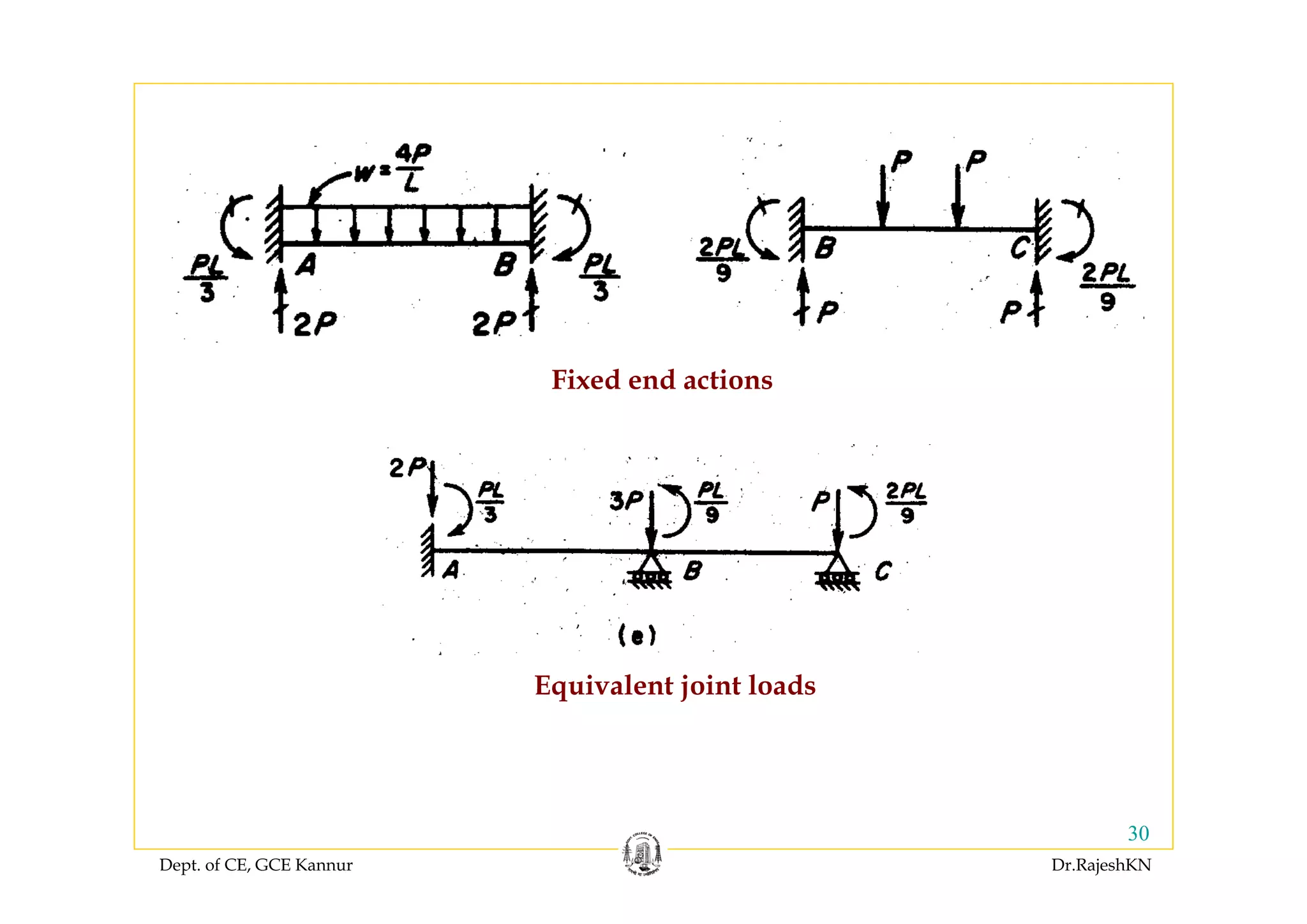
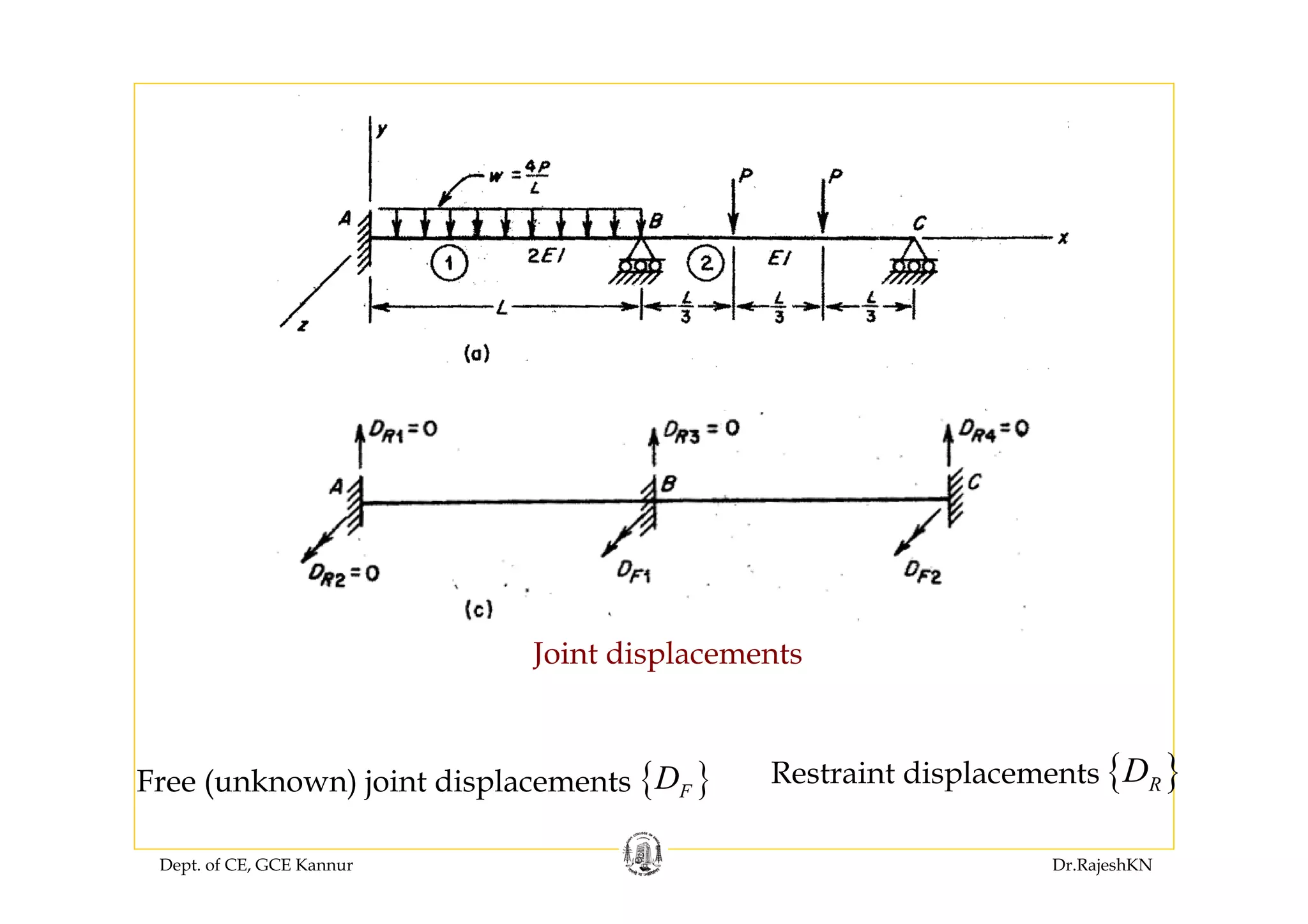
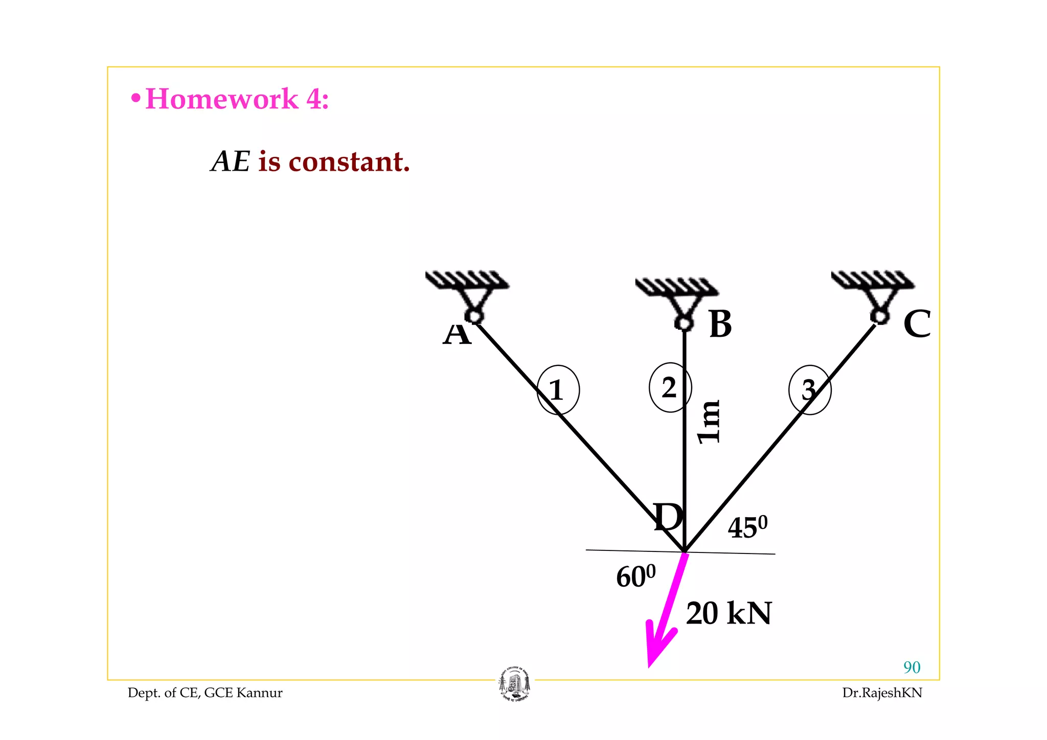
![Dept. of CE, GCE Kannur Dr.RajeshKN
•Problem 5
[ ]
2 1 0 0 0 0
1 2 0 0 0 0
0 0 2 1 0 02
0 0 1 2 0 0
0 0 0 0 2 1
0 0 0 0 1 2
M
EI
S
L
⎡ ⎤
⎢ ⎥
⎢ ⎥
⎢ ⎥
= ⎢ ⎥
⎢ ⎥
⎢ ⎥
⎢ ⎥
⎣ ⎦
Unassembled stiffness matrix](https://image.slidesharecdn.com/module2-stiffness-rajeshsir-140806045716-phpapp01/75/Module2-stiffness-rajesh-sir-73-2048.jpg)
![Dept. of CE, GCE Kannur Dr.RajeshKN
74
[ ]MFC =
0 0 1
1 0 1
1 0 0
0 1 0
0 1 1
0 0 1
L
L
L
L
⎡ ⎤
⎢ ⎥
⎢ ⎥
⎢ ⎥
⎢ ⎥
⎢ ⎥
⎢ ⎥
⎢ ⎥
⎣ ⎦
1
2
3
DF1 DF2 DF3
=1 =1 =1](https://image.slidesharecdn.com/module2-stiffness-rajeshsir-140806045716-phpapp01/75/Module2-stiffness-rajesh-sir-74-2048.jpg)
![Dept. of CE, GCE Kannur Dr.RajeshKN
75
2 1 0 0 0 0 0 0 1
1 2 0 0 0 0 1 0 1
0 1 1 0 0 0
0 0 2 1 0 0 1 0 02
0 0 0 1 1 0
0 0 1 2 0 0 0 1 0
1 1 0 0 1 1
0 0 0 0 2 1 0 1 1
0 0 0 0 1 2 0 0 1
L
L
EI
L
L L L L
L
L
⎡ ⎤ ⎡ ⎤
⎢ ⎥ ⎢ ⎥
⎢ ⎥ ⎢ ⎥⎡ ⎤
⎢ ⎥ ⎢ ⎥⎢ ⎥= ⎢ ⎥ ⎢ ⎥⎢ ⎥
⎢ ⎥ ⎢ ⎥⎢ ⎥⎣ ⎦ ⎢ ⎥ ⎢ ⎥
⎢ ⎥ ⎢ ⎥
⎣ ⎦ ⎣ ⎦
[ ] [ ] [ ][ ]T
FF MF M MFS C S C=
1 0 3
2 0 3
0 1 1 0 0 0
2 1 02
0 0 0 1 1 0
1 2 0
1 1 0 0 1 1
0 2 3
0 1 3
L
L
EI
L
L L L L
L
L
⎡ ⎤
⎢ ⎥
⎢ ⎥⎡ ⎤
⎢ ⎥⎢ ⎥= ⎢ ⎥⎢ ⎥
⎢ ⎥⎢ ⎥⎣ ⎦ ⎢ ⎥
⎢ ⎥
⎣ ⎦
2
4 1 3
2
1 4 3
3 3 12
L
EI
L
L
L L L
⎡ ⎤
⎢ ⎥=
⎢ ⎥
⎢ ⎥⎣ ⎦](https://image.slidesharecdn.com/module2-stiffness-rajeshsir-140806045716-phpapp01/75/Module2-stiffness-rajesh-sir-75-2048.jpg)
![Dept. of CE, GCE Kannur Dr.RajeshKN
76
{ } [ ] { } [ ]{ }
1
F FF F FR RD S A S D
−
= −⎡ ⎤⎣ ⎦
{ }
1
2
4 1 3 0
2
1 4 3 0
3 3 12
F
L
EI
D L
L
L L L P
−
⎛ ⎞ ⎧ ⎫⎡ ⎤
⎪ ⎪⎜ ⎟⎢ ⎥= ⎨ ⎬⎜ ⎟⎢ ⎥
⎪ ⎪⎜ ⎟⎢ ⎥ ⎩ ⎭⎣ ⎦⎝ ⎠
{ } [ ] { }
1
F FF FD S A
−
= , since there are no support displacements.
2
13 3 3 0
3 13 3 0
84
3 3 5
L
L
L
EI
L L L P
− − ⎧ ⎫⎡ ⎤
⎪ ⎪⎢ ⎥= − − ⎨ ⎬⎢ ⎥
⎪ ⎪− −⎢ ⎥ ⎩ ⎭⎣ ⎦
2
3
3
84
5
PL
EI
L
−⎧ ⎫
⎪ ⎪
−⎨ ⎬
⎪
⎩
=
⎪
⎭
Joint displacements](https://image.slidesharecdn.com/module2-stiffness-rajeshsir-140806045716-phpapp01/75/Module2-stiffness-rajesh-sir-76-2048.jpg)
![Dept. of CE, GCE Kannur Dr.RajeshKN
77
{ } { } [ ] [ ]{ } [ ]{ }( )M ML M MF F MR RA A S C D C D= + +
{ }
2
2 1 0 0 0 0 0 0 1
1 2 0 0 0 0 1 0 1
3
0 0 2 1 0 0 1 0 02
3
0 0 1 2 0 0 0 1 0 84
5
0 0 0 0 2 1 0 1 1
0 0 0 0 1 2 0 0 1
M
L
L
EI PL
A
L EI
L
L
L
⎡ ⎤ ⎡ ⎤
⎢ ⎥ ⎢ ⎥
⎢ ⎥ ⎢ ⎥ −⎧ ⎫
⎢ ⎥ ⎢ ⎥ ⎪ ⎪
= −⎨ ⎬⎢ ⎥ ⎢ ⎥
⎪ ⎪⎢ ⎥ ⎢ ⎥
⎩ ⎭⎢ ⎥ ⎢ ⎥
⎢ ⎥ ⎢ ⎥
⎣ ⎦ ⎣ ⎦
2
2 1 0 0 0 0 5
1 2 0 0 0 0 2
0 0 2 1 0 0 32
0 0 1 2 0 0 384
0 0 0 0 2 1 2
0 0 0 0 1 2 5
EI PL
L EI
⎧ ⎫⎡ ⎤
⎪ ⎪⎢ ⎥
⎪ ⎪⎢ ⎥
−⎪ ⎪⎢ ⎥
= ⎨ ⎬⎢ ⎥
−⎪ ⎪⎢ ⎥
⎪ ⎪⎢ ⎥
⎪ ⎪⎢ ⎥
⎩ ⎭⎣ ⎦
{ } [ ][ ]{ }M M MF FA S C D=
2
12
9
92
984
9
12
EI PL
L EI
⎧ ⎫
⎪ ⎪
⎪ ⎪
−⎪ ⎪
= ⎨ ⎬
−⎪ ⎪
⎪ ⎪
⎪ ⎪
⎩ ⎭
4
3
3
314
3
4
PL
⎧ ⎫
⎪ ⎪
⎪ ⎪
−
=
⎪ ⎪
⎨ ⎬
−⎪ ⎪
⎪ ⎪
⎪ ⎪
⎩ ⎭
Member end actions](https://image.slidesharecdn.com/module2-stiffness-rajeshsir-140806045716-phpapp01/75/Module2-stiffness-rajesh-sir-77-2048.jpg)
![Dept. of CE, GCE Kannur Dr.RajeshKN
78
[ ]
0.2 0.0 0.0
0.0 0.2 0.0
0.0 0.0 0.2
MS
⎡ ⎤
⎢ ⎥=
⎢ ⎥
⎢ ⎥⎣ ⎦
Unassembled stiffness matrix
•Problem 6:
1
2
3
50 kN
80 kN
5 m
5 m
5 m
4 m 4 m
3 m
3 m](https://image.slidesharecdn.com/module2-stiffness-rajeshsir-140806045716-phpapp01/75/Module2-stiffness-rajesh-sir-78-2048.jpg)
![Dept. of CE, GCE Kannur Dr.RajeshKN
[ ]MFC =
0.8 -0.6
-0.8 0.6
0.8 0.6
⎡ ⎤
⎢ ⎥
⎢ ⎥
⎢ ⎥⎣ ⎦
1
cos 36.87=0.8
36.87
1
2
3
0.8
10.6
53.13
cos 53.13=0.6
DF1 DF2
=1 =1](https://image.slidesharecdn.com/module2-stiffness-rajeshsir-140806045716-phpapp01/75/Module2-stiffness-rajesh-sir-79-2048.jpg)
![Dept. of CE, GCE Kannur Dr.RajeshKN
80
{ } [ ] { } [ ]{ }
1
F FF F FR RD S A S D
−
= −⎡ ⎤⎣ ⎦
{ }
2.930 1.302 -50
1.302 5.208 -80
FD
⎧ ⎫⎡ ⎤
= ⎨ ⎬⎢ ⎥
⎩ ⎭⎣ ⎦
{ } [ ] { }
1
F FF FD S A
−
= , since there are no support displacements.
-250.651
-481.771
⎧
=
⎫
⎨ ⎬
⎩ ⎭
Joint displacements
[ ] [ ] [ ][ ]T
FF MF M MFS C S C= 0.384 -0.096
-0.096 0.216
⎡ ⎤
= ⎢ ⎥
⎣ ⎦](https://image.slidesharecdn.com/module2-stiffness-rajeshsir-140806045716-phpapp01/75/Module2-stiffness-rajesh-sir-80-2048.jpg)
![Dept. of CE, GCE Kannur Dr.RajeshKN
0.2 0.0 0.0 0.8 -0.6
250.651
0.0 0.2 0.0 -0.8 0.6
481.771
0.0 0.0 0.2 0.8 0.6
⎡ ⎤⎡ ⎤
−⎧ ⎫⎢ ⎥⎢ ⎥= ⎨ ⎬⎢ ⎥⎢ ⎥ −⎩ ⎭
⎢ ⎥⎢ ⎥⎣ ⎦⎣ ⎦
{ } { } [ ] [ ]{ } [ ]{ }( )M ML M MF F MR RA A S C D C D= + +
[ ][ ]{ }M MF FS C D=
17.708
17.708
97.917
⎧ ⎫
⎪ ⎪
⎨−
⎪
⎩
= ⎬
− ⎪
⎭
Member Forces:](https://image.slidesharecdn.com/module2-stiffness-rajeshsir-140806045716-phpapp01/75/Module2-stiffness-rajesh-sir-81-2048.jpg)
![Dept. of CE, GCE Kannur Dr.RajeshKN
82
•Problem 7:
[ ]
0.2 0.0 0.0
0.0 0.5 0.0
0.0 0.0 0.2
MS
⎡ ⎤
⎢ ⎥=
⎢ ⎥
⎢ ⎥⎣ ⎦
Unassembled stiffness matrix
1
2
3](https://image.slidesharecdn.com/module2-stiffness-rajeshsir-140806045716-phpapp01/75/Module2-stiffness-rajesh-sir-82-2048.jpg)
![Dept. of CE, GCE Kannur Dr.RajeshKN
[ ]MFC =
0.600 0.800
0.000 -1.000
-0.600 0.800
⎡ ⎤
⎢ ⎥
⎢ ⎥
⎢ ⎥⎣ ⎦
1
53.13
5
m
cos 53.13=0.6
0.6
1
0
53.13
5
m
0
36.87
cos 36.87=0.8
cos 36.87=0.8
0.8
DF1 DF2
=1 =1](https://image.slidesharecdn.com/module2-stiffness-rajeshsir-140806045716-phpapp01/75/Module2-stiffness-rajesh-sir-83-2048.jpg)
![Dept. of CE, GCE Kannur Dr.RajeshKN
84
{ } [ ] { } [ ]{ }
1
F FF F FR RD S A S D
−
= −⎡ ⎤⎣ ⎦
{ }
6.944 0.000 15.000
0.000 1.323 -10.000
FD
⎡ ⎤ ⎧ ⎫
= ⎨ ⎬⎢ ⎥
⎣ ⎦ ⎩ ⎭
{ } [ ] { }
1
F FF FD S A
−
= , since there are no support displacements.
104.167
-13.228
⎧
=
⎫
⎨ ⎬
⎩ ⎭
Joint displacements
[ ] [ ] [ ][ ]T
FF MF M MFS C S C= 0.144 0.000
0.000 0.756
⎡ ⎤
=⎢ ⎥
⎣ ⎦](https://image.slidesharecdn.com/module2-stiffness-rajeshsir-140806045716-phpapp01/75/Module2-stiffness-rajesh-sir-84-2048.jpg)
![Dept. of CE, GCE Kannur Dr.RajeshKN
{ }
0.2 0.0 0.0 0.600 0.800
104.167
0.0 0.5 0.0 0.000 -1.000
-13.228
0.0 0.0 0.2 -0.600 0.800
MA
⎡ ⎤⎡ ⎤
⎧ ⎫⎢ ⎥⎢ ⎥= ⎨ ⎬⎢ ⎥⎢ ⎥⎩ ⎭
⎢ ⎥⎢ ⎥⎣ ⎦⎣ ⎦
{ } { } [ ] [ ]{ } [ ]{ }( )M ML M MF F MR RA A S C D C D= + +
{ } [ ][ ]{ }M M MF FA S C D=
10.4
6.6
-14.6
⎧ ⎫
⎪ ⎪
⎨ ⎬
⎪
=
⎪
⎩ ⎭
Member Forces:](https://image.slidesharecdn.com/module2-stiffness-rajeshsir-140806045716-phpapp01/75/Module2-stiffness-rajesh-sir-85-2048.jpg)
![Dept. of CE, GCE Kannur Dr.RajeshKN
[ ]
0.866 0.000 0.000
0.000 1.000 0.000
0.000 0.000 0.500
MS
⎡ ⎤
⎢ ⎥=
⎢ ⎥
⎢ ⎥⎣ ⎦
Unassembled stiffness matrix
•Problem 8 (Homework 3):](https://image.slidesharecdn.com/module2-stiffness-rajeshsir-140806045716-phpapp01/75/Module2-stiffness-rajesh-sir-86-2048.jpg)
![Dept. of CE, GCE Kannur Dr.RajeshKN
1
0.866
0.5
1
0.866
0.5
[ ]MFC =
0.866 0.500
1.000 0.000
0.500 -0.866
⎡ ⎤
⎢ ⎥
⎢ ⎥
⎢ ⎥⎣ ⎦
DF1 DF2
=1 =1](https://image.slidesharecdn.com/module2-stiffness-rajeshsir-140806045716-phpapp01/75/Module2-stiffness-rajesh-sir-87-2048.jpg)
![Dept. of CE, GCE Kannur Dr.RajeshKN
88
{ } [ ] { } [ ]{ }
1
F FF F FR RD S A S D
−
= −⎡ ⎤⎣ ⎦
{ }
0.577 -0.155 5
-0.155 1.732 0
FD
⎡ ⎤ ⎧ ⎫
= ⎨ ⎬⎢ ⎥
⎣ ⎦ ⎩ ⎭
{ } [ ] { }
1
F FF FD S A
−
= , since there are no support displacements.
2.887
-0.773
⎧ ⎫
⎨
⎩
= ⎬
⎭
Joint displacements
[ ] [ ] [ ][ ]T
FF MF M MFS C S C= 1.774 0.158
0.158 0.591
⎡ ⎤
= ⎢ ⎥
⎣ ⎦](https://image.slidesharecdn.com/module2-stiffness-rajeshsir-140806045716-phpapp01/75/Module2-stiffness-rajesh-sir-88-2048.jpg)
![Dept. of CE, GCE Kannur Dr.RajeshKN
{ }
0.866 0.000 0.000 0.866 0.500
2.887
0.000 1.000 0.000 1.000 0.000
-0.773
0.000 0.000 0.500 0.500 -0.866
MA
⎡ ⎤⎡ ⎤
⎧ ⎫⎢ ⎥⎢ ⎥= ⎨ ⎬⎢ ⎥⎢ ⎥⎩ ⎭
⎢ ⎥⎢ ⎥⎣ ⎦⎣ ⎦
{ } { } [ ] [ ]{ } [ ]{ }( )M ML M MF F MR RA A S C D C D= + +
{ } [ ][ ]{ }M M MF FA S C D=
1.830
2.887
1.057
⎧ ⎫
⎪ ⎪
⎨ ⎬
⎪ ⎪
⎩ ⎭
=
Member Forces:](https://image.slidesharecdn.com/module2-stiffness-rajeshsir-140806045716-phpapp01/75/Module2-stiffness-rajesh-sir-89-2048.jpg)

This document discusses the stiffness method for structural analysis. It begins by introducing the stiffness method and its key concepts, such as using joint displacements as the primary unknowns and establishing a relationship between member forces and displacements through stiffness matrices. It then provides examples of calculating stiffness matrices for different structural elements, including beams, trusses, frames, grids, and space frames. The document also explains how to develop the total stiffness matrix of a structure by assembling the member stiffness matrices using a displacement transformation matrix. Finally, it formalizes the stiffness method through the governing equations relating member forces, displacements, and loads.