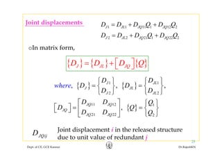
Downloaded 1,115 times
![•Generally, net deflection need not be zero
1 1 11 1 12 2Q QLD D F Q F Q= + +
D D F Q F Q+ +2 2 21 1 22 2Q QLD D F Q F Q= + +
Q Qh di l di1 2,Q QD D 1 2,Q Q•Where :support displacements corresponding to
{ } { } [ ]{ }D D F Q{ } { } [ ]{ }Q QLD D F Q= +
D⎧ ⎫ D⎧ ⎫ F F⎡ ⎤ Q⎧ ⎫
{ } 1
2
Q
Q
Q
D
D
D
⎧ ⎫
= ⎨ ⎬
⎩ ⎭
{ } 1
2
QL
QL
QL
D
D
D
⎧ ⎫
= ⎨ ⎬
⎩ ⎭
[ ] 11 12
21 22
F F
F
F F
⎡ ⎤
= ⎢ ⎥
⎣ ⎦
{ } 1
2
Q
Q
Q
⎧ ⎫
= ⎨ ⎬
⎩ ⎭
F QQDFlexibility coefficient is sometimes denoted as
Dept. of CE, GCE Kannur Dr.RajeshKN
10
F QQDFlexibility coefficient is sometimes denoted as](https://image.slidesharecdn.com/module1-flexibility-1-rajeshsir-140806045844-phpapp02/85/Module1-flexibility-1-rajesh-sir-10-320.jpg)
![{ } [ ] { } { }( )1
Q QLQ F D D
−
= −
{ } { }0D•If there are no support displacements
{ } [ ] { }1
Q F D
−
∴
{ } { }0QD =•If there are no support displacements,
{ } [ ] { }QLQ F D∴ = −
Dept. of CE, GCE Kannur Dr.RajeshKN
11](https://image.slidesharecdn.com/module1-flexibility-1-rajeshsir-140806045844-phpapp02/85/Module1-flexibility-1-rajesh-sir-11-320.jpg)
![33
11
3
L
F
EI
=
3
5L
21
5
6
L
F
EI
=
3
5L
F12
6
F
EI
=
3
22
8
3
L
F
EI
= [ ]
3
2 5
5 166
L
F
EI
⎡
=∴
⎤
⎢ ⎥
⎣ ⎦
Dept. of CE, GCE Kannur Dr.RajeshKN
14
22
3EI 5 166EI ⎣ ⎦](https://image.slidesharecdn.com/module1-flexibility-1-rajeshsir-140806045844-phpapp02/85/Module1-flexibility-1-rajesh-sir-14-320.jpg)
![⎡ ⎤
[ ]
1
3
16 56
5 27
EI
F
L
− −⎡ ⎤
= ⎢ ⎥−⎣ ⎦⎣ ⎦
Q⎡ ⎤
[ ] [ ]
11
2
QL
Q
Q F D
Q
−⎡ ⎤
⎡ ⎤= = −⎢ ⎥ ⎣ ⎦
⎣ ⎦
3
16 5 26⎡ ⎤ ⎡ ⎤ ⎡ ⎤
3
3
16 5 266
5 2 977 48
EI PL
L EI
−⎡ ⎤ ⎡ ⎤−
= ⎢ ⎥ ⎢ ⎥−⎣ ⎦ ⎣ ⎦
69
6456
P ⎡
=
⎤
⎢ ⎥−⎣ ⎦⎣ ⎦
1 2
69 8
, ,
P P
i e Q Q
−
= =
Dept. of CE, GCE Kannur Dr.RajeshKN
15
1 2. ., ,
56 7
i e Q Q](https://image.slidesharecdn.com/module1-flexibility-1-rajeshsir-140806045844-phpapp02/85/Module1-flexibility-1-rajesh-sir-15-320.jpg)
![{ } { } { } { } { } [ ]{ }{ } { } { } { } { } [ ]{ }Q QL QT QP QRD D D D D F Q= + + + +
{ } { } { } { } { }QC QL QT QP QRD D D D D= + + +•Let { } { } { } { } { }
{ } { } [ ]{ }Q QCD D F Q= +•Hence, and
{ } [ ] { } { }( )1
Q QCQ F D D
−
= −
Dept. of CE, GCE Kannur Dr.RajeshKN
17](https://image.slidesharecdn.com/module1-flexibility-1-rajeshsir-140806045844-phpapp02/85/Module1-flexibility-1-rajesh-sir-17-320.jpg)
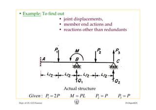
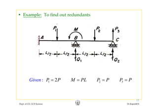
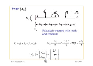
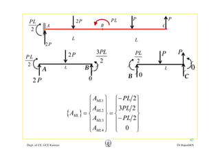
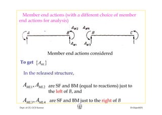
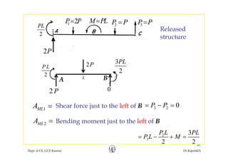
![• In the given example,In the given example,
1 2 32P P M PL P P P P= = = =
[ ]
69
64
P
Q
⎡ ⎤
= ⎢ ⎥
⎣ ⎦
As found out earlier,
Dept. of CE, GCE Kannur Dr.RajeshKN
[ ]
6456
Q ⎢ ⎥−⎣ ⎦
,](https://image.slidesharecdn.com/module1-flexibility-1-rajeshsir-140806045844-phpapp02/85/Module1-flexibility-1-rajesh-sir-30-320.jpg)
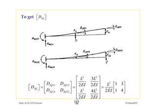
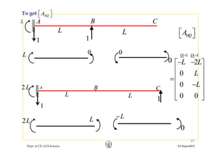
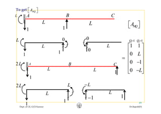
![[ ]DTo get [ ]JLDTo get
2
10PL ⎡ ⎤2
1
5
4
JL
PL
D
EI
=
2
2
13
8
JL
PL
D
EI
= [ ]
2
10
138
JL
PL
D
EI
∴
⎡ ⎤
= ⎢ ⎥
⎣ ⎦
Dept. of CE, GCE Kannur Dr.RajeshKN
32](https://image.slidesharecdn.com/module1-flexibility-1-rajeshsir-140806045844-phpapp02/85/Module1-flexibility-1-rajesh-sir-32-320.jpg)
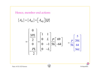
![[ ]
69P
Q
⎡ ⎤
= ⎢ ⎥Already we know [ ]
6456
Q = ⎢ ⎥−⎣ ⎦
Already we know,
Joint displacements
⎡ ⎤ ⎡ ⎤ ⎡ ⎤
{ } { } { }J JL JQD D D Q⎡ ⎤= + ⎣ ⎦
2 2
10 1 3 69
13 1 4 648 2 56
PL L P
EI EI
⎡ ⎤ ⎡ ⎤ ⎡ ⎤
= +⎢ ⎥ ⎢ ⎥ ⎢ ⎥−⎣ ⎦ ⎣ ⎦ ⎣ ⎦
2
17PL ⎡ ⎤
⎢ ⎥=
5112EI ⎢ ⎥−⎣ ⎦
=
Dept. of CE, GCE Kannur Dr.RajeshKN](https://image.slidesharecdn.com/module1-flexibility-1-rajeshsir-140806045844-phpapp02/85/Module1-flexibility-1-rajesh-sir-34-320.jpg)

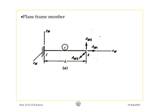
![Member flexibility matrices for prismatic members with
B b
one end fixed and the other free
3 2
L L⎡ ⎤
•Beam member
[ ] 11 12
2
21 22
3 2M M
Mi
M M
L L
F F EI EI
F
F F L L
⎡ ⎤
⎢ ⎥⎡ ⎤
⎢ ⎥= =⎢ ⎥
⎢ ⎥⎣ ⎦21 22
2
M MF F L L
EI EI
⎢ ⎥⎣ ⎦
⎢ ⎥⎣ ⎦
Dept. of CE, GCE Kannur Dr.RajeshKN](https://image.slidesharecdn.com/module1-flexibility-1-rajeshsir-140806045844-phpapp02/85/Module1-flexibility-1-rajesh-sir-52-320.jpg)
![[ ]
L
F =•Truss member [ ]MiF
EA
=•Truss member
Dept. of CE, GCE Kannur Dr.RajeshKN](https://image.slidesharecdn.com/module1-flexibility-1-rajeshsir-140806045844-phpapp02/85/Module1-flexibility-1-rajesh-sir-53-320.jpg)
![1
FM33
11 12 13 3 2
0 0
M M M
L
EA
F F F
⎡ ⎤
⎢ ⎥
⎡ ⎤ ⎢ ⎥
[ ]
11 12 13 3 2
21 22 23
231 32 33
0
3 2
M M M
Mi M M M
M M M
L L
F F F F
EI EI
F F F
L L
⎡ ⎤ ⎢ ⎥
⎢ ⎥ ⎢ ⎥= =
⎢ ⎥ ⎢ ⎥
⎢ ⎥ ⎢ ⎥⎣ ⎦
Dept. of CE, GCE Kannur Dr.RajeshKN
231 32 33
0
2
M M M
L L
EI EI
⎢ ⎥ ⎢ ⎥⎣ ⎦
⎢ ⎥
⎢ ⎥⎣ ⎦](https://image.slidesharecdn.com/module1-flexibility-1-rajeshsir-140806045844-phpapp02/85/Module1-flexibility-1-rajesh-sir-55-320.jpg)
![FM31
FM33
3 2
L L⎡ ⎤
[ ]
11 12 13
0
3 2
M M M
L L
EI EIF F F
L
⎡ ⎤
⎢ ⎥
⎡ ⎤ ⎢ ⎥
⎢ ⎥ ⎢ ⎥
[ ] 21 22 23
231 32 33
0 0Mi M M M
M M M
L
F F F F
GJ
F F F
L L
⎢ ⎥ ⎢ ⎥= =
⎢ ⎥ ⎢ ⎥
⎢ ⎥ ⎢ ⎥⎣ ⎦
⎢ ⎥
Dept. of CE, GCE Kannur Dr.RajeshKN
0
2
L L
EI EI
⎢ ⎥
⎢ ⎥⎣ ⎦](https://image.slidesharecdn.com/module1-flexibility-1-rajeshsir-140806045844-phpapp02/85/Module1-flexibility-1-rajesh-sir-57-320.jpg)
![0 0 0 0 0
L
E A
⎡ ⎤
⎢ ⎥
⎢ ⎥3 2
0 0 0 0
3 2Z Z
E A
L L
E I E I
⎢ ⎥
⎢ ⎥
⎢ ⎥
⎢ ⎥
[ ]
3 2
0 0 0 0
3 2
Z Z
Y Y
L L
E I E I
F
⎢ ⎥
−⎢ ⎥
⎢ ⎥
⎢ ⎥[ ]
0 0 0 0 0
M iF
L
G J
⎢ ⎥=
⎢ ⎥
⎢ ⎥
⎢ ⎥2
0 0 0 0
2 Y Y
L L
E I E I
⎢ ⎥
−⎢ ⎥
⎢ ⎥
⎢ ⎥2
0 0 0 0
2 Z Z
L L
E I E I
⎢ ⎥
⎢ ⎥
⎢ ⎥
⎣ ⎦
Dept. of CE, GCE Kannur Dr.RajeshKN](https://image.slidesharecdn.com/module1-flexibility-1-rajeshsir-140806045844-phpapp02/85/Module1-flexibility-1-rajesh-sir-59-320.jpg)
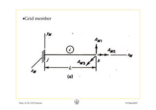
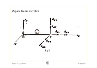
![Formalization of the Flexibility method
(Explanation using principle of complimentary virtual work)
{ } [ ]{ }D F A
For each member,
{ } [ ]{ }Mi Mi MiD F A=
contains relative displacements of the k end{ }DH contains relative displacements of the k end
with respect to j end of the i-th member
{ }MiDHere
Dept. of CE, GCE Kannur Dr.RajeshKN](https://image.slidesharecdn.com/module1-flexibility-1-rajeshsir-140806045844-phpapp02/85/Module1-flexibility-1-rajesh-sir-60-320.jpg)
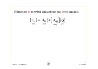
![•If there are m members in the structure,
{ } [ ] [ ] [ ] [ ] [ ] { }11 10 0 0 0MM MFD A⎧ ⎫ ⎧ ⎫⎡ ⎤
⎪ ⎪ ⎪ ⎪⎢ ⎥
{ }
{ }
[ ] [ ] [ ] [ ] [ ]
[ ] [ ] [ ] [ ] [ ]
{ }
{ }
22 2
33 3
0 0 0 0
0 0 0 0
MM M
MM M
FD A
FD A
⎪ ⎪ ⎪ ⎪⎢ ⎥
⎪ ⎪ ⎪ ⎪⎢ ⎥
⎪ ⎪ ⎪ ⎪⎢ ⎥
⎪ ⎪ ⎪ ⎪⎢ ⎥
{ } [ ] [ ] [ ] [ ] [ ] { }0 0 0 0MiMi MiFD A
⎪ ⎪ ⎪ ⎪⎢ ⎥
=⎨ ⎬ ⎨ ⎬⎢ ⎥
⎪ ⎪ ⎪ ⎪⎢ ⎥
⎪ ⎪ ⎪ ⎪⎢ ⎥
{ } [ ] [ ] [ ] [ ] [ ] { }0 0 0 0 MmMm MmFD A
⎪ ⎪ ⎪ ⎪⎢ ⎥
⎪ ⎪ ⎪ ⎪⎢ ⎥
⎪ ⎪ ⎪ ⎪⎢ ⎥
⎩ ⎭ ⎩ ⎭⎣ ⎦
{ } [ ]{ }D F A
Dept. of CE, GCE Kannur Dr.RajeshKN
{ } [ ]{ }M M MD F A=](https://image.slidesharecdn.com/module1-flexibility-1-rajeshsir-140806045844-phpapp02/85/Module1-flexibility-1-rajesh-sir-61-320.jpg)
![{ } [ ]{ }M M MD F A={ } [ ]{ }M M M
[ ]MF is the unassembled flexibility matrix of the entire structure
{ }MA
{ }A
•Member end actions in will be related to the
structure actions applied to the released structure
{ }SA { }JA { }QAconsists of joint loads and redundant actions
{ }SAstructure actions applied to the released structure.
{ }S { }J { }Qj
{ } [ ]{ }M MS SA B A=Hence,
A i f i iAction transformation matrix
(equilibrium matrix)
{ } [ ]
{ }
{ }
J
M MJ MQ
A
A B B
⎧ ⎫⎪ ⎪⎡ ⎤⎡ ⎤= ⎨ ⎬⎣ ⎦⎣ ⎦
i.e.,
Dept. of CE, GCE Kannur Dr.RajeshKN
{ } [ ]
{ }M MJ MQ
QA
⎨ ⎬⎣ ⎦⎣ ⎦
⎪ ⎪⎩ ⎭](https://image.slidesharecdn.com/module1-flexibility-1-rajeshsir-140806045844-phpapp02/85/Module1-flexibility-1-rajesh-sir-62-320.jpg)
![[ ]B { }A { }A andl t to[ ]MJB
MQB⎡ ⎤⎣ ⎦
{ }MA { }JA
{ }QA
andrelate to
relate to{ }MA
•Each column in the submatrix consists of[ ]MJB
MQB⎡ ⎤⎣ ⎦ { }Qrelate { }M
•Each column in the submatrix consists of
member end actions caused by a unit value of a joint
load applied to the released structure.
[ ]MJB
pp
•Each column in the submatrix consists of
member end actions caused by a unit value of a
MQB⎡ ⎤⎣ ⎦
member end actions caused by a unit value of a
redundant applied to the released structure.
Dept. of CE, GCE Kannur Dr.RajeshKN](https://image.slidesharecdn.com/module1-flexibility-1-rajeshsir-140806045844-phpapp02/85/Module1-flexibility-1-rajesh-sir-63-320.jpg)
![{ }SAδ•Suppose an arbitrary set of virtual actions { }SSuppose an arbitrary set of virtual actions
is applied on the structure.
{ } [ ]{ } [ ]
{ }
{ }
J
M MS S MJ MQ
A
A B A B B
A
δ
δ δ
δ
⎧ ⎫⎪ ⎪⎡ ⎤⎡ ⎤= = ⎨ ⎬⎣ ⎦⎣ ⎦
⎪ ⎪⎩ ⎭
{ } [ ]{ } [ ]
{ }Q
QAδ⎣ ⎦⎣ ⎦
⎪ ⎪⎩ ⎭
External complimentary virtual work produced by the
{ }SAδ { }SD
External complimentary virtual work produced by the
virtual loads and actual displacements is
{ } { } { } { }
TT T* JD
W A D A Aδ δ δ δ
⎧ ⎫⎡ ⎤ ⎨ ⎬{ } { } { } { }T T J
S S J Q
Q
W A D A A
D
δ δ δ δ⎡ ⎤= = ⎨ ⎬⎢ ⎥⎣ ⎦ ⎩ ⎭
Dept. of CE, GCE Kannur Dr.RajeshKN](https://image.slidesharecdn.com/module1-flexibility-1-rajeshsir-140806045844-phpapp02/85/Module1-flexibility-1-rajesh-sir-64-320.jpg)
![•Equating the above two (principle of complimentary
i t l k)
{ } { } { } { }
T T
S S M MA D A Dδ δ=
virtual work),
{ } { } { } { }S S M MA D A Dδ δ
{ } [ ]{ }{ } [ ]{ }A A { } [ ]{ }M M MD F A={ } [ ]{ }M MS SA B A=But and
{ } [ ]{ }M MS SA B Aδ δ=Also,
{ } { } { } [ ] [ ][ ]{ }
TT T
S S S MS M MS SA D A B F B Aδ δ=Hence, { } { } { } [ ] [ ][ ]{ }S S S MS M MS S
Dept. of CE, GCE Kannur Dr.RajeshKN](https://image.slidesharecdn.com/module1-flexibility-1-rajeshsir-140806045844-phpapp02/85/Module1-flexibility-1-rajesh-sir-66-320.jpg)
![{ } [ ] [ ][ ]{ }
T
D B F B A{ } [ ] [ ][ ]{ }S MS M MS SD B F B A=
{ } [ ]{ }S S SD F A=
[ ] [ ] [ ][ ]
T
F B F B
Where,
the assembled flexibility matrix
[ ] [ ] [ ][ ]
T
S MS M MSF B F B= , the assembled flexibility matrix
for the entire structure.
Dept. of CE, GCE Kannur Dr.RajeshKN](https://image.slidesharecdn.com/module1-flexibility-1-rajeshsir-140806045844-phpapp02/85/Module1-flexibility-1-rajesh-sir-67-320.jpg)
![[ ]SF is partitioned into submatrices related to:[ ]S
{ }JA
p
joint loads
{ }QAand redundant actions
{ } [ ]{ }
{ } [ ] { }JJ JQJ J
F FD A
A
⎡ ⎤⎡ ⎤⎧ ⎫ ⎧ ⎫⎪ ⎪ ⎣ ⎦ ⎪ ⎪⎢ ⎥⎨ ⎬ ⎨ ⎬{ } [ ]{ }
{ }
{ }
[ ] { }
{ }
QJ J
Q QQJ
S S S
QQ
D
D AF F
F A
⎪ ⎪ ⎣ ⎦ ⎪ ⎪⎢ ⎥=⎨ ⎬ ⎨ ⎬
⎢ ⎥⎡ ⎤ ⎡ ⎤⎪ ⎪ ⎪ ⎪⎩ ⎭ ⎩ ⎭⎣ ⎦
=
⎣ ⎦⎣ ⎦
⇒
T T
⎡ ⎤ ⎡ ⎤
Where,
[ ] [ ] [ ][ ]
T
JJ MJ M MJF B F B= [ ] [ ]
T
JQ MJ M MQF B F B⎡ ⎤ ⎡ ⎤=⎣ ⎦ ⎣ ⎦
T
⎡ ⎤ ⎡ ⎤
T
⎡ ⎤ ⎡ ⎤ ⎡ ⎤
Dept. of CE, GCE Kannur Dr.RajeshKN
[ ][ ]
T
QJ MQ M MJF B F B⎡ ⎤ ⎡ ⎤=⎣ ⎦ ⎣ ⎦ [ ]
T
QQ MQ M MQF B F B⎡ ⎤ ⎡ ⎤ ⎡ ⎤=⎣ ⎦ ⎣ ⎦ ⎣ ⎦](https://image.slidesharecdn.com/module1-flexibility-1-rajeshsir-140806045844-phpapp02/85/Module1-flexibility-1-rajesh-sir-68-320.jpg)
![{ } [ ]{ } { }D F A F A⎡ ⎤= + ⎣ ⎦{ } [ ]{ } { }J JJ J JQ QD F A F A⎡ ⎤= + ⎣ ⎦
{ } { } { }D F A F A⎡ ⎤ ⎡ ⎤= +⎣ ⎦ ⎣ ⎦{ } { } { }Q QJ J QQ QD F A F A⎡ ⎤ ⎡ ⎤= +⎣ ⎦ ⎣ ⎦
1
{ } { } { }
1
Q QQ Q QJ JA F D F A
−
⎡ ⎤⎡ ⎤ ⎡ ⎤= −⎣ ⎦ ⎣ ⎦⎣⇒ ⎦
Dept. of CE, GCE Kannur Dr.RajeshKN](https://image.slidesharecdn.com/module1-flexibility-1-rajeshsir-140806045844-phpapp02/85/Module1-flexibility-1-rajesh-sir-69-320.jpg)
![{ }{ }QA
{ }JD
• Once redundants are found,
can be found out from,
{ } [ ]{ } { }D F A F A⎡ ⎤+ ⎣ ⎦
{ }J ,
{ } [ ]{ } { }J JJ J JQ QD F A F A⎡ ⎤= + ⎣ ⎦
Dept. of CE, GCE Kannur Dr.RajeshKN
71](https://image.slidesharecdn.com/module1-flexibility-1-rajeshsir-140806045844-phpapp02/85/Module1-flexibility-1-rajesh-sir-71-320.jpg)
![• Similarly, support reactions caused by joint loads and
redundant can be obtained with an action transformation
matrix [ ]RSB[ ]RS
{ } [ ]{ } [ ]
{ }JA⎧ ⎫⎪ ⎪⎡ ⎤⎡ ⎤{ } [ ]{ } [ ]
{ }
{ }
J
R RS S RJ RQ
Q
A B A B B
A
⎪ ⎪⎡ ⎤⎡ ⎤= = ⎨ ⎬⎣ ⎦⎣ ⎦
⎪ ⎪⎩ ⎭
•Each column in the submatrix consists of support
i d b i l f j i l d li d
[ ]RJB
reactions caused by a unit value of a joint load applied to
the released structure.
B⎡ ⎤RQB⎡ ⎤⎣ ⎦•Each column in the submatrix consists of
support reactions caused by a unit value of a
Dept. of CE, GCE Kannur Dr.RajeshKN
pp y
redundant applied to the released structure.](https://image.slidesharecdn.com/module1-flexibility-1-rajeshsir-140806045844-phpapp02/85/Module1-flexibility-1-rajesh-sir-72-320.jpg)
![• If actual or equivalent joint loads are applied• If actual or equivalent joint loads are applied
directly to the supports,
{ } { } [ ]{ } { }R RC RJ J RQ QA A B A B A⎡ ⎤= − + + ⎣ ⎦
t bi d j i t l d ( t l d
{ }RCA
represents combined joint loads (actual and
equivalent) applied directly to the supports.
Dept. of CE, GCE Kannur Dr.RajeshKN](https://image.slidesharecdn.com/module1-flexibility-1-rajeshsir-140806045844-phpapp02/85/Module1-flexibility-1-rajesh-sir-73-320.jpg)
![•As seen earlier, member end actions due to actual loads,
are obtained by superimposing member end actions due
to restraint actions and combined joint loads
{ } { } [ ]{ } { }M MF MJ J MQ QA A B A B A⎡ ⎤= + + ⎣ ⎦{ } { } [ ]{ } { }M MF MJ J MQ Q⎣ ⎦
{ }Awhere represents fixed end actions{ }MFAwhere represents fixed end actions
Dept. of CE, GCE Kannur Dr.RajeshKN](https://image.slidesharecdn.com/module1-flexibility-1-rajeshsir-140806045844-phpapp02/85/Module1-flexibility-1-rajesh-sir-74-320.jpg)
![Comparison of the procedures explained with principle
of superposition and principle of complimentary virtual
work
•For calculating redundants,
{ } [ ] { } { }( )1
Q F D D
−
P i i l f iti
Principle of complimentary virtual work
{ } [ ] { } { }( )Q QLQ F D D= −Principle of superposition
{ } { } { }
1
Q QQ Q QJ JA F D F A
−
⎡ ⎤⎡ ⎤ ⎡ ⎤= −⎣ ⎦ ⎣ ⎦⎣ ⎦
Principle of complimentary virtual work
{ } { } { }Q QQ Q QJ J⎣ ⎦ ⎣ ⎦⎣ ⎦
[ ]F F⎡ ⎤⎣ ⎦H [ ] QQF F⎡ ⎤= ⎣ ⎦Hence,
{ } { }D F A⎡ ⎤d{ } { }Q A
Dept. of CE, GCE Kannur Dr.RajeshKN
{ } { }QL QJ JD F A⎡ ⎤= ⎣ ⎦and{ } { }QQ A=](https://image.slidesharecdn.com/module1-flexibility-1-rajeshsir-140806045844-phpapp02/85/Module1-flexibility-1-rajesh-sir-75-320.jpg)
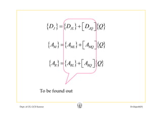
![•For calculating joint displacements,g j p
{ } { } { }J JL JQD D D Q⎡ ⎤= + ⎣ ⎦
Principle of superposition
Principle of complimentary virtual work
{ } [ ]{ } { }J JJ J JQ QD F A F A⎡ ⎤= + ⎣ ⎦
{ } [ ]{ }JL JJ JD F A=Hence and{ } [ ]{ }JL JJ JD F A
JQ JQD F⎡ ⎤ ⎡ ⎤=⎣ ⎦ ⎣ ⎦
Hence, and
Q Q⎣ ⎦ ⎣ ⎦
Dept. of CE, GCE Kannur Dr.RajeshKN](https://image.slidesharecdn.com/module1-flexibility-1-rajeshsir-140806045844-phpapp02/85/Module1-flexibility-1-rajesh-sir-76-320.jpg)
![•For calculating member end actions,g ,
{ } { } { }M ML MQA A A Q⎡ ⎤= + ⎣ ⎦Principle of superposition
Principle of complimentary virtual work
{ } { } [ ]{ } { }M MF MJ J MQ QA A B A B A⎡ ⎤= + + ⎣ ⎦
{ } { } [ ]{ }ML MF MJ JA A B A= +Hence, and
MQ MQA B⎡ ⎤ ⎡ ⎤=⎣ ⎦ ⎣ ⎦
Dept. of CE, GCE Kannur Dr.RajeshKN](https://image.slidesharecdn.com/module1-flexibility-1-rajeshsir-140806045844-phpapp02/85/Module1-flexibility-1-rajesh-sir-77-320.jpg)
![•For calculating support reactions•For calculating support reactions,
{ } { } { }R RL RQA A A Q⎡ ⎤= +⎣ ⎦Principle of superposition
Principle of complimentary virtual work
{ } { } { }R RL RQ Q⎣ ⎦p p p
{ } { } [ ]{ } { }R RC RJ J RQ QA A B A B A⎡ ⎤= − + + ⎣ ⎦
{ } { } [ ]{ }RL RC RJ JA A B A= − +Hence, and
RQ RQA B⎡ ⎤ ⎡ ⎤=⎣ ⎦ ⎣ ⎦
Dept. of CE, GCE Kannur Dr.RajeshKN](https://image.slidesharecdn.com/module1-flexibility-1-rajeshsir-140806045844-phpapp02/85/Module1-flexibility-1-rajesh-sir-78-320.jpg)
![Similarly,
L
F
L
F
−
1
11
3
MF
EI
=12
6
MF
EI
=
11 12 3 6
L L
F F EI EI
−⎡ ⎤
⎢ ⎥⎡ ⎤
[ ] 11 12
21 22
3 6
6 3
M M
Mi
M M
F F EI EI
F
F F L L
EI EI
⎢ ⎥⎡ ⎤
∴ = = ⎢ ⎥⎢ ⎥ −⎣ ⎦ ⎢ ⎥
⎢ ⎥⎣ ⎦
Dept. of CE, GCE Kannur Dr.RajeshKN
81
6 3EI EI⎢ ⎥⎣ ⎦](https://image.slidesharecdn.com/module1-flexibility-1-rajeshsir-140806045844-phpapp02/85/Module1-flexibility-1-rajesh-sir-81-320.jpg)
![Member flexibility matrix for a beam member with
t d h t d b d timoment and shear at one end as member end actions
3 2
L L
F F
⎡ ⎤
⎢ ⎥⎡ ⎤
[ ] 11 12
2
21 22
3 2M M
Mi
M M
F F EI EI
F
F F L L
⎢ ⎥⎡ ⎤
⎢ ⎥= =⎢ ⎥
⎢ ⎥⎣ ⎦
⎢ ⎥
Dept. of CE, GCE Kannur Dr.RajeshKN
2EI EI⎢ ⎥⎣ ⎦](https://image.slidesharecdn.com/module1-flexibility-1-rajeshsir-140806045844-phpapp02/85/Module1-flexibility-1-rajesh-sir-82-320.jpg)


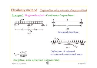
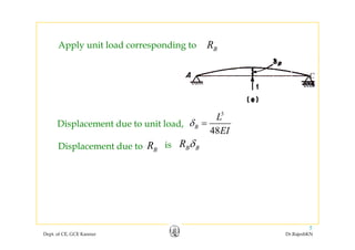
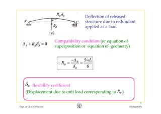
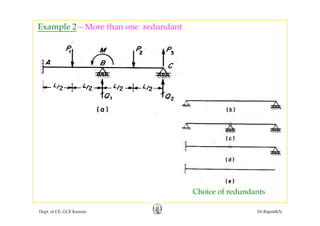
This document discusses the flexibility method for structural analysis. The flexibility method involves determining flexibility coefficients by applying unit loads corresponding to redundant forces and calculating the resulting displacements. These flexibility coefficients are then used to calculate the redundant forces needed to satisfy compatibility conditions. The flexibility matrices for different structural elements are developed. Joint displacements, member end actions, and support reactions can be determined by incorporating the flexibility coefficients into the basic computations. Examples are provided to illustrate the flexibility method for a continuous beam with one redundant and for determining various outputs like redundants, joint displacements, and reactions.