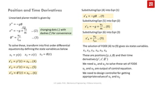
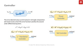
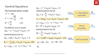
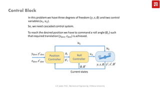
This document describes modeling and controller design for a quadcopter. It begins by developing a 1D model of the quadcopter as a single degree of freedom system. It then expands this to a nonlinear 6 degree of freedom model and linearizes it about hover conditions. The document derives state space representations of the linearized models. Finally, it describes designing separate controllers for translation, thrust, and roll based on satisfying second order differential equations for the errors between desired and actual states.

![1D Model of Quadcopter
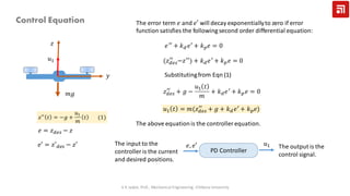
𝑚 ሷ𝑧 𝑡 = 𝑢 𝑡 − 𝑚𝑔
𝑥1 = 𝑧(𝑡)
𝑥2 = ሶ𝑧 t
changing variables into state variables:
𝑢 𝑡 = 𝑢1
= ሶ𝑥1
In state-space modelling, we want to see the dynamics
of the each states.
ሶ𝑥1 = 𝑥2 ሶ𝑥2 =
1
𝑚
𝑢1 − 𝑔
Two initialconditionsare required to solve these first
order differential equationson the state; 𝑥1(0) and 𝑥2(0).
𝑥1 0 = 𝑧 0 = 0 𝑥2 0 = ሶ𝑧 0 = 0
𝑚𝑔
𝑏2
𝑏3
𝑎2
𝑎3
𝑢1
𝑧 = 𝑧 𝑑𝑒𝑠
scipy.integrate.odeint(func, y0, t, args=(), tfirst=False)
Function model
V K Jadon, Prof., Mechanical Engineering, Chitkara University
def model(z,t,u):
x1=z[0] # Intial Conditionfor First
FODE
x2=z[1] # Initial conditionfor
Second FODE
dx1dt=x2 # First FODE
dx2dt=(u-c*x2-k*x1)/mass-gravity # Second FODE
dxdt = [dx1dt,dx2dt]
return dxdt](https://image.slidesharecdn.com/session-viquadmodel-200110053538/85/quadcopter-modelling-and-controller-design-3-320.jpg)
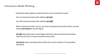
![time=np.linspace(0,1,10)
sol = odeint(model, [displacement,velocity], time)
#Initial Conditions
displacement=0, velocity=0
#System Parameters
k=0, c=0, g=9.81, mass=0.18
#System Input
u1=10
𝑘 = 0, 𝑐 = 0, 𝑔 = 9.81, 𝑚𝑎𝑠𝑠 = 0.18
𝑑 = 0; 𝑣 = 0; 𝑢1 = 0
𝑑 = 1; 𝑣 = 0;
𝑢1 = 0
𝑑 = 0; 𝑣 = 0;
𝑢1 = 1
𝑘 = 0, 𝑐 = 0, 𝑔 = 9.81, 𝑚𝑎𝑠𝑠 = 0.18
𝑘 = 0, 𝑐 = 0, 𝑔 = 9.81, 𝑚𝑎𝑠𝑠 = 0.18
𝑘 = 0, 𝑐 = 0, 𝑔 = 9.81, 𝑚𝑎𝑠𝑠 = 0.18
𝑑 = 0; 𝑣 = 5;
𝑢1 = 0
1D SODE Response
V K Jadon, Prof., Mechanical Engineering, Chitkara University
def model(z,t,u):
x1=z[0]
x2=z[1]
dx1dt=x2
dx2dt=(u-c*x2-k*x1)/mass-gravity
dxdt = [dx1dt,dx2dt]
return dxdt](https://image.slidesharecdn.com/session-viquadmodel-200110053538/85/quadcopter-modelling-and-controller-design-4-320.jpg)