Download as PDF, PPTX
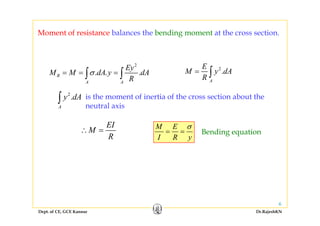
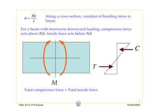
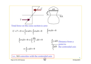
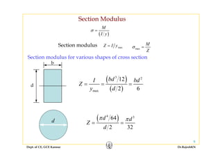
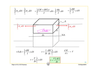
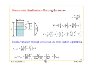
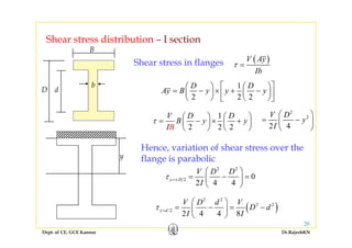
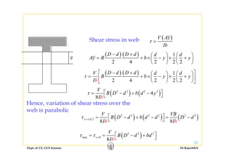
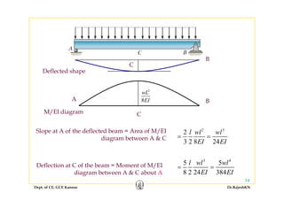
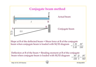
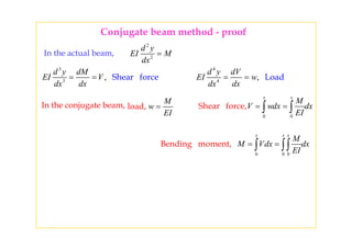
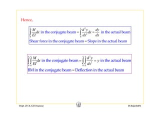
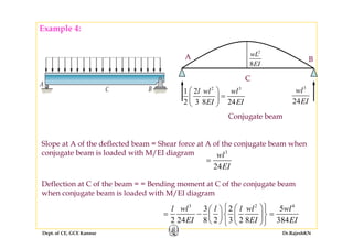

This document discusses stresses in beams, including: 1) Bending stresses in beams, shear flow, and shearing stress formulae for beams. 2) Inelastic bending of beams and deflection of beams using various calculation methods. 3) Elementary treatment of statically indeterminate beams like fixed and continuous beams. It provides theories, formulae, and examples for calculating stresses in beams undergoing bending loads.