
More Related Content
What's hot
What's hot (20)
Similar to Mechanics of Quadcopter
Similar to Mechanics of Quadcopter (20)
More from Vijay Kumar Jadon
More from Vijay Kumar Jadon (14)
Recently uploaded
Recently uploaded (20)
Mechanics of Quadcopter
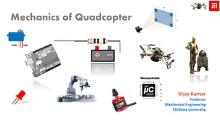
- 1. Vijay Kumar Professor Mechanical Engineering Chitkara University Mechanics of Quadcopter
- 2. V. K. Jadon, Prof., Mechanical Engineering, Chitkara University Motor Mixing Dynamics of Drone The Flow …. Rotation Kinematics
- 3. Vectors A vector has magnitude and direction. 𝐴′ 𝐵′ 𝐴 𝐵 Both vectors represents same quantity 𝒂 𝒃 Commutative Law 𝒂 𝒃 𝒃 𝒂 𝒂 + 𝒃 = 𝒃 + 𝒂 Associative Law 𝒄 𝒂 𝒃 𝒂 + 𝒃 + 𝒄 = 𝒂 + (𝒃 + 𝒄) Addition Subtraction 𝒂 𝒃 −𝒃 𝒂 V K Jadon, Professor, Mechanical Engineering, Chitkara University
- 4. Vector Components 𝒂 𝑎 𝑥 𝑎 𝑦 𝜃 A component of a vector is the projection of the vector on an axis. 𝑥 𝑦 𝒂 𝑎 𝑥 𝑎 𝑦 𝜃 𝑥 𝑦 Shifting a vector without changing its direction does not change its components. Using right angle triangle 𝑎 𝑥 = 𝑎𝑐𝑜𝑠𝜃 𝑎 𝑦 = 𝑎𝑠𝑖𝑛𝜃 Vector 𝒂 is given by 𝑎 and 𝜃. Vector 𝒂 is given by 𝑎 𝑥 and 𝑎 𝑦. 𝑎 = 𝑎 𝑥 2 + 𝑎 𝑦 2 Vector 𝒂 can be transformed into magnitude-angle notation 𝑡𝑎𝑛𝜃 = 𝑎 𝑦 𝑎 𝑥 For 3D case, we need a magnitude and two angles or three components to represent a vector V K Jadon, Professor, Mechanical Engineering, Chitkara University
- 5. Unit Vector A unit vector has unit magnitude 𝒊, 𝒋, 𝒌 are the unit vectors along x, y and z axes respectively. These are used to express any vector. 𝒂 𝑎 𝑥 𝑎 𝑦 𝜃 𝑥 𝑦 𝒂 = 𝑎 𝑥 𝒊 + 𝑎 𝑦 𝒋 𝒂 = 𝑎 𝑥 𝒊 + 𝑎 𝑦 𝒋 + 𝑎 𝑧 𝒌 𝒃 = 𝑏 𝑥 𝒊 + 𝑏 𝑦 𝒋 + 𝑏 𝑧 𝒌 𝑖𝑓 𝒓 = 𝒂 + 𝒃 𝑟𝑥 = 𝑎 𝑥 + 𝑏 𝑥 𝑟𝑦 = 𝑎 𝑦 + 𝑏 𝑦 𝑟𝑧 = 𝑎 𝑧 + 𝑏 𝑧 𝒂 𝑎 𝑥 𝑎 𝑦 𝜃 𝑥 𝑦 𝑎 = 𝑎 𝑥 2 + 𝑎 𝑦 2 𝒓 = 𝑟𝑥 𝒊 + 𝑟𝑦 𝒋 + 𝑟𝑧 𝒌 V K Jadon, Professor, Mechanical Engineering, Chitkara University
- 6. 𝒂 = 𝑎 𝑥 𝒊 + 𝑎 𝑦 𝒋 + 𝑎 𝑧 𝒌 𝑎 𝑥 𝑎 𝑦 𝑥 𝑦 𝑎 𝑧 Vector in Space 𝑧 In matrix form 𝒂 = 𝑎 𝑥 𝑎 𝑦 𝑎 𝑧 𝒂 = 𝐴 𝑥 𝐴 𝑦 𝐴 𝑧 𝑤 Modified form to include scale factor Where 𝑎 𝑥 = 𝐴 𝑥 𝑤 𝑎 𝑦 = 𝐴 𝑦 𝑤 𝑎 𝑧 = 𝐴 𝑧 𝑤 If 𝑤 > 1 scale up If 𝑤 < 1 scale down 𝑤 = 0 means components are infinite. It represents only the direction of the vector. V K Jadon, Professor, Mechanical Engineering, Chitkara University
- 7. Multiplication of Vectors Scalar Product is regarded as product of magnitude of one vector and the scalar component of the second vector along the direction of first vector. 𝒂 𝜃 𝒃 𝒂 .𝒃 = 𝑎 (𝑏 𝑐𝑜𝑠𝜃) 𝒂 𝜃 𝒃 𝑎 𝑐𝑜𝑠𝜃 𝒂 .𝒃 = 𝑏 (𝑎 𝑐𝑜𝑠𝜃) 𝒂 = 𝑎 𝑥 𝒊 + 𝑎 𝑦 𝒋 + 𝑎 𝑧 𝒌 𝒃 = 𝑏 𝑥 𝒊 + 𝑏 𝑦 𝒋 + 𝑏 𝑧 𝒌 𝒂. 𝒃 = 𝑎 𝑥 𝑏 𝑥 + 𝑎 𝑦 𝑏 𝑦 + 𝑎 𝑧 𝑏 𝑧 What is the angle between 3.0𝒊 − 4.0𝒋 and −2.0𝒊 + 3.0𝒌 V K Jadon, Professor, Mechanical Engineering, Chitkara University
- 8. Multiplication of Vectors Vector Product of two vectors produces another vector whose magnitude is 𝑎𝑏 𝑠𝑖𝑛𝜃 and acts along perpendicular to the plane that contains the two vectors. 𝒂 𝜃 𝒃 𝒄 = 𝒂 × 𝒃 = 𝑎 𝑏 𝑠𝑖𝑛𝜃 𝒄 𝒂 = 𝑎 𝑥 𝒊 + 𝑎 𝑦 𝒋 + 𝑎 𝑧 𝒌 𝒃 = 𝑏 𝑥 𝒊 + 𝑏 𝑦 𝒋 + 𝑏 𝑧 𝒌 𝒂 × 𝒃 = (𝑎 𝑦 𝑏 𝑧 − 𝑏 𝑦 𝑎 𝑧)𝒊 + (𝑎 𝑧 𝑏 𝑥 − 𝑏 𝑧 𝑎 𝑥)𝒋 +(𝑎 𝑥 𝑏 𝑦 − 𝑏 𝑥 𝑎 𝑦)𝒌 𝒂 𝜃 𝒃 𝒄 = 𝒃 × 𝒂 = 𝑎 𝑏 𝑠𝑖𝑛𝜃 A vector lies in xy plane, has magnitude of 18 units and points in a direction 250 from the positive direction of x, Also, vector b has magnitude of 12 units and points along the positive direction of z. what is the vector product. V K Jadon, Professor, Mechanical Engineering, Chitkara University
- 9. Linear Velocity 𝑶 𝑥 𝑦 𝐴 𝑡 = 𝑡 𝐴 𝑡 = 𝑡 𝐵 What is the direction of velocity of particle when 𝑡 > 0; 𝑡 ≤ 𝑡 𝐴 ? What is the direction of velocity of particle when 𝑡 > 𝑡 𝐴; 𝑡 ≤ 𝑡 𝐵 ? What is the velocity of particle when 𝑡 = 𝑡 𝐵 ? What is the direction of velocity of particle when 𝑡 = 𝑡 𝐵 ? 𝐵 𝒓 𝒗 𝑩 ∆𝒕 = lim ∆𝑡→0 ∆𝒔 ∆𝑡 = 𝑑𝒔 𝑑𝑡 𝒗 𝑩 𝒂𝒗𝒈 = 𝑑𝒓 𝑑𝑡 V K Jadon, Professor, Mechanical Engineering, Chitkara University
- 10. 𝑶 𝑥 𝑦 𝑧 rotation about x-axis 𝑶 𝑥 𝑦 𝑧 𝜃 𝑥 = 900 𝜃 𝑥 𝜃 𝑦 𝜃 𝑦 = 900 𝑶 𝑥 𝑦 𝑧 rotation about y-axis Angular Displacement 𝜃 𝑦 = 900 𝑶 𝑥 𝑦 𝑧 rotation about y-axis rotation about x-axis 𝜃 𝑥 = 900 𝜃 𝑦 𝑶 𝑥 𝑦 𝑧 𝜽 𝒙 + 𝜽 𝒚 ≠ 𝜽 𝒚 + 𝜽 𝒙 𝜃 𝑥 𝝎 = lim ∆𝜽→𝟎 ∆𝜽 ∆𝒕 Direction is given by Right Hand Rule ∆𝜽 𝒙 + ∆𝜽 𝒚 = ∆𝜽 𝒚 + ∆𝜽 𝒙 V K Jadon, Professor, Mechanical Engineering, Chitkara University Commutative Law not valid
- 11. Velocity and Acceleration 𝑶 𝑥 𝑦 𝑃 𝜔 𝒗 𝒑 = 𝑑(𝒓) 𝑑𝑡 = 𝝎 × 𝒓 𝝎 = 𝜔 𝒌 𝒓 = 𝑟 𝒓 𝒌 × 𝒓 = 𝒓 𝜽 Where 𝒌, 𝒓 𝑎𝑛𝑑 𝒓 𝜽 constitute a right hand coordinate system 𝑨 𝒑 = 𝑑(𝒗 𝒑) 𝑑𝑡 = 𝑑(𝝎 × 𝒓 ) 𝑑𝑡 If 𝝎 is constant = 𝝎 × 𝑑𝒓 𝑑𝑡 + 𝑑𝝎 𝑑𝑡 × 𝒓 𝑨 𝒑 = 𝝎 × 𝑑𝒓 𝑑𝑡 = 𝝎 × 𝑟 𝑑 𝒓 𝑑𝑡 𝑑(𝒓) 𝑑𝑡 = 𝑟 𝑑( 𝒓) 𝑑𝑡 = 𝑟(𝝎 × 𝒓) 𝑑𝝎 𝑑𝑡 = 0 = 𝝎 × 𝑟(𝝎 × 𝒓) = 𝝎 × (𝝎 × 𝒓) If 𝝎 changes with time 𝑨 𝒑 = 𝝎 × 𝝎 × 𝒓 + 𝛂 × 𝒓 𝒓 Magnitude 𝑟 does not change V K Jadon, Professor, Mechanical Engineering, Chitkara University
- 12. Vector in Rotated Frame 𝒂 = 𝑎 𝑥 𝒊 + 𝑎 𝑦 𝒋 𝑦′ 𝑥′ 𝑎 𝑦 ′ 𝑎 𝑥 ′ 𝒂 𝑎 𝑥 𝑎 𝑦 𝑥 𝑦 𝒂 𝑎 𝑥 𝑎 𝑦 𝑥 𝑦 𝒂 = 𝑎 𝑥 𝒊 + 𝑎 𝑦 𝒋 𝒂 = 𝑎 𝑥 ′ 𝒊′ + 𝑎 𝑦 ′ 𝒋′ V K Jadon, Professor, Mechanical Engineering, Chitkara University
- 13. Rigid body Rotation 𝒂 𝑎 𝑥 𝑎 𝑦 𝑥 𝑦 𝒂 = 𝑎 𝑥 𝒊 + 𝑎 𝑦 𝒋 𝒂′ = 𝑎 𝑥 ′′ 𝒊 + 𝑎 𝑦 ′′ 𝒋 𝒂 = 𝑎 𝑥 𝒊 + 𝑎 𝑦 𝒋 𝒂′ = 𝑎 𝑥 𝒊′ + 𝑎 𝑦 𝒋′ 𝑃 𝑦′ 𝑥′ 𝒂′ 𝑎 𝑦 𝑎 𝑥 𝜃 𝑃 Position vector 𝒂 of point 𝑃 in a rigid body Position vector 𝒂′ of point 𝑃 in a rigid body after rotation of rigid body about origin Overlapping two positions of rigid body before and after rotation. 𝑦′ 𝑥′ 𝑎 𝑦 ′ 𝑎 𝑥 ′ 𝒂 𝑎 𝑥 𝑎 𝑦 𝜃 𝑥 𝑦 𝒂′ 𝑃 𝑃′ 𝑎 𝑦 ′′ 𝑎 𝑥 ′′ 𝒂′ = 𝑎 𝑥 𝒊′ + 𝑎 𝑦 𝒋′ Rotated 𝑃 becomes 𝑃′ V K Jadon, Professor, Mechanical Engineering, Chitkara University
- 14. Rigid body Rotation 𝒂 = 𝑎 𝑥 𝒊 + 𝑎 𝑦 𝒋 𝒂′ = 𝑎 𝑥 ′′ 𝒊 + 𝑎 𝑦 ′′ 𝒋 𝑦′ 𝑥′ 𝑎 𝑦 ′ 𝑎 𝑥 ′ 𝒂 𝑎 𝑥 𝑎 𝑦 𝜃 𝑥 𝑦 𝒂′ 𝑃 𝑃′ 𝑎 𝑦 ′′ 𝑎 𝑥 ′′ 𝒂′ = 𝑎 𝑥 𝒊′ + 𝑎 𝑦 𝒋′ In matrix form 𝒂 = 𝑎 𝑥 𝑎 𝑦 𝒊 𝒋 𝒂′ = 𝑎′′ 𝑥 𝑎′′ 𝑦 𝒊 𝒋 𝒂 = 𝑎 𝑇 𝒖 𝑎 𝑇 = 𝑎 𝑥 𝑎 𝑦 𝒂′ = 𝑎′′ 𝑇 𝒖 𝑎′ 𝑇 = 𝑎′′ 𝑥 𝑎′′ 𝑦 𝒂′ = 𝑎 𝑥 𝑎 𝑦 𝒊′′ 𝒋′′ 𝒂′ = 𝑎 𝑇 𝒖′ 𝑎 𝑇 = 𝑎 𝑥 𝑎 𝑦 𝒙 − 𝒂𝒙𝒊𝒔 𝒚 − 𝒂𝒙𝒊𝒔 𝑎 𝑥 𝑎 𝑦 𝒙′ − 𝒂𝒙𝒊𝒔 𝒚′ − 𝒂𝒙𝒊𝒔 𝑎′ 𝑥 𝑎′ 𝑦 Projection of 𝒂 𝑜𝑛 Projection of 𝒂′ 𝑜𝑛 𝒙 − 𝒂𝒙𝒊𝒔 𝒚 − 𝒂𝒙𝒊𝒔 𝑎′′ 𝑥 𝑎′′ 𝑦 Projection of 𝒂′ 𝑜𝑛 Our aim is to find projections of rotated vectors on reference axes system in terms of the projections of original vector on reference axis. To find 𝑎′′ 𝑥, 𝑎′′ 𝑦 in terms of 𝑎 𝑥, 𝑎 𝑦 V K Jadon, Professor, Mechanical Engineering, Chitkara University
- 15. 𝑥0 Body Fixed Frame in Reference Frame 𝑦0 𝑧0 𝑥1 𝑦1 𝑧1 𝐹 = 𝑥1𝑥𝑜 𝑦1𝑥0 𝑧1𝑥0 𝑥1𝑦0 𝑦1𝑦0 𝑧1𝑦0 𝑥1𝑧0 𝑦1𝑧0 𝑧1𝑧0 𝑥0 𝑦0 𝑧0 𝑥1 𝑦1 𝑧1 V K Jadon, Professor, Mechanical Engineering, Chitkara University
- 16. 𝑦′ 𝑥′ 𝑝 𝑥 𝑝 𝑦 𝜃 𝑥 𝑦 𝑃 𝑃′ Pure Rotation about an axes To find 𝑝 𝑥, 𝑝 𝑦 in terms of 𝑝 𝑥′ and 𝑝 𝑦′ 𝒙 − 𝒂𝒙𝒊𝒔 𝒚 − 𝒂𝒙𝒊𝒔 𝑝 𝑥 𝑝 𝑦 𝒙′ − 𝒂𝒙𝒊𝒔 𝒚′ − 𝒂𝒙𝒊𝒔 𝑝 𝑥 𝑝 𝑦 Projection of 𝑷 𝑜𝑛 Projection of 𝑷′ 𝑜𝑛 𝒙 − 𝒂𝒙𝒊𝒔 𝒚 − 𝒂𝒙𝒊𝒔 𝑝 𝑥′ 𝑝 𝑦′ Projection of 𝑷′ 𝑜𝑛 𝑝 𝑥 = projection of 𝑃′ along 𝒙 reference axis 𝑝 𝑥′ 𝑝 𝑦′ 𝑝 𝑦 = projection of 𝑃′ along 𝑦 reference axis 𝑝 𝑥′ = projection of 𝑃′ along 𝒙′ body fixed axis 𝑝 𝑦′ = projection of 𝑃′ along 𝒚′ body fixed axis V K Jadon, Professor, Mechanical Engineering, Chitkara University
- 17. 𝑂𝐴 = 𝑝 𝑥 𝑂𝐵 = 𝑝 𝑦 𝜃 𝑃′ Pure Rotation about an axes 𝑂𝐶 = 𝑝 𝑥′ 𝑂𝐷 = 𝑝 𝑦′ 𝑥 𝑦 𝑂 𝐶 𝐴 𝐵 𝐷 𝐸 𝐹 𝑝 𝑥 = 𝑂𝐴 = 𝑂𝐸 − 𝐴𝐸 …(i) 𝑂𝐸 = 𝑂𝐶 𝑐𝑜𝑠𝜃 = 𝑝 𝑥′ 𝑐𝑜𝑠𝜃 𝐴𝐸 = 𝐶𝐺 𝐺 = 𝐶𝑃′ 𝑠𝑖𝑛𝜃 = 𝑝 𝑦′ 𝑠𝑖𝑛𝜃 𝑝 𝑥 = 𝑝 𝑥′ 𝑐𝑜𝑠𝜃 − 𝑝 𝑦′ 𝑠𝑖𝑛𝜃 𝑝 𝑦 = 𝑂𝐵 = 𝑂𝐹 + 𝐹𝐵 …(ii) 𝑂𝐹 = 𝑂𝐷 𝑐𝑜𝑠𝜃 = 𝑝 𝑦′ 𝑐𝑜𝑠𝜃 𝑝 𝑦 = 𝑝 𝑥′ 𝑠𝑖𝑛𝜃 + 𝑝 𝑦′ 𝑐𝑜𝑠𝜃 𝑝 𝑥 𝑝 𝑦 = 𝑐𝑜𝑠𝜃 −𝑠𝑖𝑛𝜃 𝑠𝑖𝑛𝜃 𝑐𝑜𝑠𝜃 𝑝 𝑥′ 𝑝 𝑦′ Vector 𝒑 in reference frame is obtained if we multiply vector 𝒑 in body frame (rotated fame) by rotation matrix. 𝒑 𝑥𝑦 = 𝑅(𝑧, 𝜃)𝒑 𝑥′ 𝑦′ 𝑐𝑜𝑠𝜃 −𝑠𝑖𝑛𝜃 𝑠𝑖𝑛𝜃 𝑐𝑜𝑠𝜃 Projection of unit vector of 𝑥′ Projection of unit vector of 𝑦′ On unit vector of 𝑥 On unit vector of 𝑦 𝐻 𝐹𝐵 = 𝐻𝑃′ = 𝐷𝑃′ 𝑠𝑖𝑛𝜃 = 𝑝 𝑥′ 𝑐𝑜𝑠𝜃 V K Jadon, Professor, Mechanical Engineering, Chitkara University
- 18. 𝜃 Pure Rotation about an axes (3D) 𝑝 𝑥 𝑝 𝑦 𝑝 𝑧 = 𝑐𝑜𝑠𝜃 −𝑠𝑖𝑛𝜃 0 𝑠𝑖𝑛𝜃 𝑐𝑜𝑠𝜃 0 0 0 1 𝑝 𝑥′ 𝑝 𝑦′ 𝑝 𝑧′ Vector 𝒑 in reference frame is obtained if we multiply vector 𝒑 in body frame (rotated fame) by rotation matrix. 𝒑 𝑥𝑦𝑧 = 𝑅(𝑧, 𝜃)𝒑 𝑥′ 𝑦′ 𝑧′ Projection of unit vector of 𝑥′ Projection of unit vector of 𝑧′ On unit vector of 𝑥 On unit vector of 𝑦 𝑥 𝑦 𝑂 𝑧 𝑃′ On unit vector of 𝑧 𝑐𝑜𝑠𝜃 −𝑠𝑖𝑛𝜃 0 𝑠𝑖𝑛𝜃 𝑐𝑜𝑠𝜃 0 0 0 1 Projection of unit vector of 𝑦′ 𝑝 𝑥 𝑝 𝑦 𝑝 𝑧 = 𝐶𝜃 −𝑆𝜃 0 𝑆𝜃 𝐶𝜃 0 0 0 1 𝑝 𝑥′ 𝑝 𝑦′ 𝑝 𝑧′ 𝑅(𝑧, 𝜃) V K Jadon, Professor, Mechanical Engineering, Chitkara University
- 19. Rotation Matrix of 3D Frames 𝒙 𝟎 𝒛 𝟎 𝒚 𝟎 𝒙 𝟏 𝒚 𝟏 𝒛 𝟏 𝑝 𝑥 𝑞 𝑥 𝑟𝑥 𝑝 𝑦 𝑞 𝑦 𝑟𝑦 𝑝 𝑧 𝑞 𝑧 𝑟𝑧 [𝑅1 0 ] = 𝒙 𝟏 𝒚 𝟏 𝒛 𝟏 𝒙 𝟎 𝒚 𝟎 𝒛 𝟎 Rotation about 𝑧 − 𝑎𝑥𝑖𝑠 𝐶𝜃 −𝑆𝜃 0 𝑆𝜃 𝐶𝜃 0 0 0 1 [𝑅1𝑧 0 ] = 𝒙 𝟏 𝒚 𝟏 𝒛 𝟏 𝒙 𝟎 𝒚 𝟎 𝒛 𝟎 Rotation about 𝑥 − 𝑎𝑥𝑖𝑠 1 0 0 0 𝐶𝜃 −𝑆𝜃 0 𝑆𝜃 𝐶𝜃 [𝑅1𝑥 0 ] = 𝒙 𝟏 𝒚 𝟏 𝒛 𝟏 𝒙 𝟎 𝒚 𝟎 𝒛 𝟎 𝒙 𝟏𝒛 𝟏 𝒚 𝟏 𝐶𝜃 0 𝑆𝜃 0 1 0 −𝑆𝜃 0 𝐶𝜃 [𝑅1𝑦 0 ] = 𝒙 𝟏 𝒚 𝟏 𝒛 𝟏 𝒙 𝟎 𝒚 𝟎 𝒛 𝟎 𝒙 𝟏 𝒛 𝟏 𝒚 𝟏 𝒙 𝟏 𝒚 𝟏 𝒛 𝟏 Rotation about y − 𝑎𝑥𝑖𝑠 𝑝 𝑥, 𝑝 𝑦, 𝑝 𝑧 represent the components of vector 𝒙 𝟏 V K Jadon, Professor, Mechanical Engineering, Chitkara University
- 20. = 1 0 0 0 cos(180) −sin(180) 0 sin(180) cos 180 𝑅 𝑐 𝐹 = 𝒙 𝒄 𝒚 𝒄 𝒛 𝒄 𝒙 𝒄 𝒚 𝒄 𝒛 𝒄 𝒙 𝒄 𝒚 𝒄 𝒛 𝒄 𝒙 𝒄 𝒚 𝒄 𝒛 𝒄 Rotation about 𝑥 − 𝑎𝑥𝑖𝑠 Rotation about 𝑧 − 𝑎𝑥𝑖𝑠 cos(−90) −sin(−90) 0 sin(−90) cos(−90) 0 0 0 1 𝑅 𝑐𝑥 1 𝑅 𝑐𝑧 2 Initial Position of frame Final Position of frame = 1 0 0 0 −1 0 0 0 −1 0 1 0 −1 0 0 0 0 1 = 0 1 0 1 0 0 0 0 −1 V K Jadon, Professor, Mechanical Engineering, Chitkara University Pure Rotation about an axes (3D)
- 21. A point 𝒑 2,3,4 is marked to a rigid body. The body is rotated by 900 about 𝑥 − 𝑎𝑥𝑖𝑠 of the reference frame. Find the coordinate of point 𝑤. 𝑟. 𝑡. reference axis. 𝑝 𝑥 𝑝 𝑦 𝑝 𝑧 = 1 0 0 0 𝐶𝜃 −𝑆𝜃 0 𝑆𝜃 𝐶𝜃 𝑝 𝑥′ 𝑝 𝑦′ 𝑝 𝑧′ 𝑅(𝑥, 𝜃) 𝑥0 𝑦0 𝑧0 𝒑 2,3,4 𝑝 𝑥 𝑝 𝑦 𝑝 𝑧 = 1 0 0 0 0 −1 0 1 0 2 3 4 𝑝 𝑥 𝑝 𝑦 𝑝 𝑧 = 2 1 + 3(0) + 4(0) 2 0 + 3 0 + 4(−1) 2 0 + 3 1 + 4(0) = 2 −4 3 𝑥1 𝑦1 𝑧1 V K Jadon, Professor, Mechanical Engineering, Chitkara University
- 22. 𝑻𝒐 𝒑𝒓𝒐𝒗𝒆 𝒑𝒙 = 𝒑𝒙′ 𝒄𝒐𝒔𝜽 − 𝒑𝒚′ 𝒔𝒊𝒏𝜽 & 𝒑𝒚 = 𝒑𝒙′ 𝒔𝒊𝒏𝜽 + 𝒑𝒚′ 𝒄𝒐𝒔𝜽 𝑰𝒏 ∆𝑶𝑫𝑬 𝐷𝐸 𝑂𝐷 = 𝑡𝑎𝑛𝜃 𝐷𝐸 = 𝑂𝐷𝑡𝑎𝑛𝜃 = 𝑝𝑦; 𝑡𝑎𝑛𝜃 ∆𝑂𝐷𝐸 & ∆𝑝𝐵𝐶 ∆𝐷𝐸 ~ ∆𝑝𝐵𝐶 𝐷𝐸 = 𝐵𝐶 = 𝑝𝑦′ 𝑡𝑎𝑛𝜃 𝑂𝐵 = 𝑂𝐶 + 𝐵𝐶 𝑂𝐶 = 𝑂𝐵 − 𝐵𝐶 𝑂𝐶 = 𝑝𝑥′ − 𝑝𝑦′ 𝑡𝑎𝑛𝜃 𝑰𝒏 ∆𝑶𝑨𝑪 𝑂𝐴 𝑂𝐶 = 𝑐𝑜𝑠𝜃 = 𝑂𝐴 = 𝑂𝐶𝑐𝑜𝑠𝜃 p𝑥 = 𝑝𝑥′ − 𝑝𝑦′ 𝑡𝑎𝑛𝜃 𝑐𝑜𝑠𝜃 = 𝑝𝑥′ 𝑐𝑜𝑠𝜃 − 𝑝𝑦′ 𝑠𝑖𝑛𝜃 𝑐𝑜𝑠𝜃 × 𝑐𝑜𝑠𝜃 𝒚 𝒙 𝒙′ 𝒑′ 𝟎 𝒚′ 𝒄 𝑥, 𝑦 𝒑𝒚′ 𝜃 𝑩 𝜃 Alternate Solution-Derived by one of Student Jaskaran Singh V K Jadon, Professor, Mechanical Engineering, Chitkara University
- 23. 𝑵𝒐𝒘 𝑰𝒏 ∆𝑶𝑫𝑬 𝑂𝐷 𝑂𝐸 = 𝑐𝑜𝑠𝜃 𝑂𝐸 = 𝑂𝐷 𝑐𝑜𝑠𝜃 = 𝑝𝑦′ 𝑐𝑜𝑠𝜃 𝑰𝒏 ∆𝑷𝑬𝑭 𝐸𝐹 = 𝑝𝐹𝑡𝑎𝑛𝜃 𝑂𝐸 + 𝐸𝐹 = 𝑝𝑦 p 𝑦 = 𝑝𝑦′ 𝑐𝑜𝑠𝜃 + 𝑝𝑥′ 𝑐𝑜𝑠𝜃 − 𝑝𝑦′ 𝑠𝑖𝑛𝜃 𝑡𝑎𝑛𝜃 p𝑦 = 𝑝𝑦′ 𝑐𝑜𝑠𝜃 + 𝑝𝑥′ 𝑐𝑜𝑠𝜃 ×𝑠𝑖𝑛𝜃 𝑐𝑜𝑠𝜃 − 𝑝𝑦′ 𝑠𝑖𝑛𝜃 ×𝑠𝑖𝑛𝜃 𝑐𝑜𝑠𝜃 𝑝𝑦 = 𝑝𝑥′ 𝑠𝑖𝑛𝜃 + 𝑝𝑦′ 𝑐𝑜𝑠𝜃 − 𝑝𝑦′ 𝑠𝑖𝑛2 𝜃 𝑐𝑜𝑠𝜃 p𝑦 = 𝑝𝑥′ 𝑠𝑖𝑛𝜃 + 𝑝𝑦′ 1 − 𝑠𝑖𝑛2 𝜃 𝑐𝑜𝑠𝜃 p𝑦 = 𝑝𝑥′ 𝑠𝑖𝑛𝜃 + 𝑝𝑦′ 𝑐𝑜𝑠2 𝜃 𝑐𝑜𝑠𝜃 V K Jadon, Professor, Mechanical Engineering, Chitkara University
- 24. Fundamental of Fluids Laminar flow Fluid flows in layers which does not cross each other. Turbulent flow The path traced by fluid particles crosses each other due to high velocity and low viscosity Compressible Flow Density changes during the flow Incompressible Flow Density remains constant Steady flow Flow parameters such as pressure, velocity etc. does not change w.r.t. time Unsteady flow Flow parameters change w.r.t. time Continuity equation Bernoulli’s Equation Mass flow rate is constant at every cross section. 𝜌𝐴𝑣 = 𝑐𝑜𝑛𝑠𝑡𝑎𝑛𝑡 𝜌1 𝐴1 𝑣1 = 𝜌2 𝐴2 𝑣2 compressible flow 𝐴1 𝑣1 = 𝐴2 𝑣2 incompressible flow 𝑝 𝜌𝑔 + 𝑣2 2𝑔 + 𝑍 = 𝑐𝑜𝑛𝑠𝑡𝑎𝑛𝑡 𝑝 𝜌𝑔 static pressure head 𝑣2 2𝑔 dynamic pressure head 𝑍 datum head 𝑝1 𝜌𝑔 + 𝑣1 2 2𝑔 + 𝑍1 = 𝑝2 𝜌𝑔 + 𝑣2 2 2𝑔 + 𝑍2 V K Jadon, Professor, Mechanical Engineering, Chitkara University
- 25. −𝑣𝑒 𝑝𝑠𝑡𝑎𝑡𝑖𝑐 +𝑣𝑒 𝑝𝑠𝑡𝑎𝑡𝑖𝑐 Dynamic pressure difference is responsible for Drag. Static pressure difference is responsible for Lift. More flow velocity is required at the top region of aerofoil compared to bottom to reach at a particular point. Due to this, the dynamic pressure increases at top region and static pressure decreases. Due to this low static pressure, the upward force (lift) is created. 1 2 Thrust 𝐿𝑒𝑎𝑑𝑖𝑛𝑔 𝐸𝑑𝑔𝑒 𝑇𝑟𝑎𝑖𝑙𝑖𝑛𝑔 𝐸𝑑𝑔𝑒 𝑀𝑎𝑥𝑖𝑚𝑢𝑚 𝐶𝑎𝑚𝑏𝑒𝑟 𝐶𝑎𝑚𝑏𝑒𝑟 𝐿𝑖𝑛𝑒 𝐶ℎ𝑜𝑟𝑑 𝐿𝑖𝑛𝑒 V K Jadon, Professor, Mechanical Engineering, Chitkara University
- 26. Quadcopter Dynamics 1 23 4 𝜔1 𝜔2𝜔3 𝜔4 𝒙𝒚 𝒛 𝑀2 𝑀1 𝑀4 𝑀3 𝐹2𝐹3 𝐹1𝐹4 V K Jadon, Professor, Mechanical Engineering, Chitkara University
- 27. Quadcopter Dynamics 𝑀2 𝑀1 𝑀4 𝑀3 𝐹2𝐹3 𝐹1𝐹4 One for each degree of freedom 𝑥 − Translation along x-axis 𝜓 − Rotation about x-axis 𝑦 − Translation along y-axis 𝑧 − Translation along x-axis ∅ − Rotation about y-axis 𝜃 − Rotation about z-axis 𝜓, ∅, 𝜃 are known as Euler Angles 𝜓, ∅, 𝜃 are called as Roll, Pitch, and Yaw Angles Forward and backward Left and Right Up and Down 𝐹1, 𝐹2, 𝐹3, 𝐹4 thrust force at rotors 1, 2, 3, 4 respectively 𝑀1, 𝑀2, 𝑀3, 𝑀4 moment reaction at rotors 1, 2, 3, 4 respectively Six equations to describe the motion of Quadcopter Six degrees of freedom 𝒙 𝒚 𝒛 V K Jadon, Professor, Mechanical Engineering, Chitkara University
- 28. 𝑀2 𝑀1 𝑀4 𝑀3 𝐹2𝐹3 𝐹1𝐹4 Force and Moment Resultant force on the quadrotor 𝑭 = 𝑭 𝟏+ 𝑭 𝟐+ 𝑭 𝟑+ 𝑭 𝟒 − 𝑚𝑔𝒌 Resultant moment on the quadrotor 𝑴 = 𝒓 𝟏 × 𝑭 𝟏 + 𝒓 𝟐 × 𝑭 𝟐 + 𝒓 𝟑 × 𝑭 𝟑 + 𝒓 𝟒 × 𝑭 𝟒 +𝑴 𝟏 + 𝑴 𝟐 + 𝑴 𝟑 + 𝑴 𝟒 𝒙 𝒚 𝒛 V K Jadon, Professor, Mechanical Engineering, Chitkara University
- 29. 𝑀2 𝑀1 𝑀4 𝑀3 𝐹2𝐹3 𝐹1 𝐹4 Upward motion 𝐹𝑧 > 𝐹1𝑧+ 𝐹2𝑧+ 𝐹3𝑧+ 𝐹4𝑧 − 𝑚𝑔 Downward motion 𝐹𝑧 > 𝐹1𝑧+ 𝐹2𝑧+ 𝐹3𝑧+ 𝐹4𝑧 − 𝑚𝑔 Hovering motion 𝐹𝑧 > 𝐹1𝑧+ 𝐹2𝑧+ 𝐹3𝑧+ 𝐹4𝑧 − 𝑚𝑔 𝑭 𝑚𝑔 𝑭 𝑚𝑔 𝑭 𝑚𝑔 𝒙 𝒚 𝑀 𝑥 = 𝑟(𝐹1 + 𝐹2) − 𝑟(𝐹3 + 𝐹4) = 0 𝒛 𝒚 𝜓 = 0 ∅ = 0𝑀 𝑦 = 𝑟(𝐹1 + 𝐹4) − 𝑟(𝐹2 + 𝐹3) = 0 𝜃 = 0𝑀𝑧 = 𝑀1 + 𝑀3 − 𝑀2 − 𝑀4 = 0 V K Jadon, Professor, Mechanical Engineering, Chitkara University
- 30. 𝑀2 𝑀1 𝑀4 𝑀3 𝐹2 𝐹3 𝐹1𝐹4 Left/Right Translation: Rolling 𝐹𝑦 = (𝐹1+ 𝐹2+ 𝐹3+ 𝐹4) sin 𝜓 𝑭 𝑚𝑔 𝐹1 + 𝐹2 𝐹3 + 𝐹4 𝑀 𝑥 𝒙 𝒚 𝒛 𝒚𝜓 𝐹𝑦 = 𝑚 𝑦 𝐹𝑧 = (𝐹1+ 𝐹2+ 𝐹3+ 𝐹4) cos 𝜓 𝐹𝑧 = 𝑚𝑔 𝑀 𝑥 = 𝐼 𝑥 𝜓 𝑧 = 𝑐𝑜𝑛𝑠𝑡𝑎𝑛𝑡 Rolling𝒛 𝒚 𝐹𝑦 𝐹𝑧 𝑀 𝑦 = 𝑀𝑧 = 0 V K Jadon, Professor, Mechanical Engineering, Chitkara University
- 31. 𝑀2 𝑀1 𝑀4 𝑀3 𝐹2 𝐹3 𝐹1 𝐹4 Forward/Backward Translation : Pitching 𝐹𝑥 = (𝐹1+ 𝐹2+ 𝐹3+ 𝐹4) sin ∅ 𝑭 𝑚𝑔𝐹1 + 𝐹4 𝐹2 + 𝐹3 𝑀 𝑦 𝒙 𝒚 𝐹𝑥 = 𝑚 𝑥 𝐹𝑧 = (𝐹1+ 𝐹2+ 𝐹3+ 𝐹4) cos ∅ 𝐹𝑧 = 𝑚𝑔 𝑀 𝑦 = 𝐼 𝑦∅ 𝑧 = 𝑐𝑜𝑛𝑠𝑡𝑎𝑛𝑡 Pitching 𝒙 𝒛 ∅ 𝐹𝑧 𝑀 𝑥 = 𝑀𝑧 = 0 V K Jadon, Professor, Mechanical Engineering, Chitkara University
- 32. 𝑀2 𝑀1 𝑀4 𝑀3 𝐹2𝐹3 𝐹1𝐹4 Yawing 𝒙 𝒚 𝐹𝑧 = (𝐹1+ 𝐹2+ 𝐹3+ 𝐹4) 𝐹𝑧 = 𝑚𝑔 𝑀𝑧 = 𝐼𝑧 𝜃 𝑧 = 𝑐𝑜𝑛𝑠𝑡𝑎𝑛𝑡 Yawing 𝒛 𝒚 𝑀2 𝑀1 𝑀4 𝑀3 𝐹2𝐹3 𝐹1𝐹4 𝑀 𝑥 = 𝑀 𝑦 = 0 𝑀 𝑥 ≠ 0 V K Jadon, Professor, Mechanical Engineering, Chitkara University
- 33. 𝑀𝑜𝑡𝑜𝑟𝐹𝑟𝑜𝑛𝑡 𝑅𝑖𝑔ℎ𝑡 𝑀𝑜𝑡𝑜𝑟𝐹𝑟𝑜𝑛𝑡 𝐿𝑒𝑓𝑡 𝑀𝑜𝑡𝑜𝑟𝐵𝑎𝑐𝑘 𝐿𝑒𝑓𝑡 𝑀𝑜𝑡𝑜𝑟𝐵𝑎𝑐𝑘 𝑅𝑖𝑔ℎ𝑡 𝑻𝒓𝒖𝒔𝒕 𝑀2 𝑀1 𝑀4 𝑀3 𝐹2𝐹3 𝐹1 𝐹4 𝒙 𝒚 𝒛 𝒚 𝒀𝒂𝒘 𝑀2 𝑀3 𝑀1 𝑀4 𝑷𝒊𝒕𝒄𝒉 𝑹𝒐𝒍𝒍 Motor Commands V K Jadon, Professor, Mechanical Engineering, Chitkara University
- 34. Sensors SystemState Controller Reference State 𝑀1 𝑀2 𝑀3 𝑀4 Controller compute the motor command to achieve the desired state Control Block Diagram 𝒆𝒓𝒓𝒐𝒓 V K Jadon, Professor, Mechanical Engineering, Chitkara University
- 35. Quadcopter Dynamics 𝒙 𝒚 𝑀2 𝑀1𝑀4 𝑀3 𝐹2𝐹3 𝐹1𝐹4 𝑇ℎ𝑟𝑢𝑠𝑡 𝑟𝑝𝑚 𝐹 = 𝑘 𝐹 𝜔2 𝐷𝑟𝑎𝑔 𝑀𝑜𝑚𝑒𝑛𝑡 𝑀 = 𝑘 𝑀 𝜔2 𝑤0 = 1 4 𝑚𝑔 𝑤0 𝜔0 𝑇 Resultant force on the quadrotor 𝑭 = 𝑭 𝟏+ 𝑭 𝟐+ 𝑭 𝟑+ 𝑭 𝟒 − 𝑚𝑔𝒌 Resultant moment on the quadrotor 𝑴 = 𝒓 𝟏 × 𝑭 𝟏 + 𝒓 𝟐 × 𝑭 𝟐 +𝑴 𝟏 + 𝑴 𝟐 + 𝑴 𝟑 + 𝑴 𝟒 +𝒓 𝟑 × 𝑭 𝟑 + 𝒓 𝟒 × 𝑭 𝟒 V K Jadon, Professor, Mechanical Engineering, Chitkara University
- 36. 𝑎2 𝑎3 𝑎1 𝑏2 𝑏3 𝑏1 𝑎1 𝑎2 𝑎3 𝐼𝑛𝑒𝑟𝑡𝑖𝑎𝑙 𝐹𝑟𝑎𝑚𝑒 𝑏1 𝑏2 𝑏3 𝐵𝑜𝑑𝑦 𝐹𝑖𝑥𝑒𝑑 𝐹𝑟𝑎𝑚𝑒 𝑭 = 𝑑𝑳 𝑪 𝑩 𝑑𝑡 𝐴 𝑖𝑠 𝑡ℎ𝑒 𝑟𝑎𝑡𝑒 𝑜𝑓 𝑐ℎ𝑎𝑛𝑔𝑒 𝑜𝑓 𝐿𝑖𝑛𝑒𝑎𝑟 𝑚𝑜𝑚𝑒𝑛𝑡𝑢𝑚 𝑖𝑛 𝑖𝑛𝑒𝑟𝑡𝑖𝑎𝑙 𝑓𝑟𝑎𝑚𝑒 𝑴 𝑪 𝑩 𝐴 = 𝑑𝑯 𝑪 𝑩 𝑑𝑡 𝐴 𝑖𝑠 𝑡ℎ𝑒 𝑟𝑎𝑡𝑒 𝑜𝑓 𝑐ℎ𝑎𝑛𝑔𝑒 𝑜𝑓 𝑎𝑛𝑔𝑢𝑙𝑎𝑟 𝑚𝑜𝑚𝑒𝑛𝑡𝑢𝑚 𝑖𝑛 𝑖𝑛𝑒𝑟𝑡𝑖𝑎𝑙 𝑓𝑟𝑎𝑚𝑒 𝑯 𝑪 𝑩 𝐴 = 𝐼 𝐶 𝝎 𝑨 𝑩 𝐼 𝐶 𝝎 𝑨 𝑩 Angular momentum of body B with respect to A. It is a 3D vector 𝑯 𝑪 𝑩 𝐴 Angular velocity of body B with respect to A. It is a 3D vector Inertia tensor with CG of the body as center Quadcopter Dynamics V K Jadon, Professor, Mechanical Engineering, Chitkara University 𝑑𝑷 𝑪 𝑩 𝑑𝑡 𝐴 = 𝑑𝑷 𝑪 𝑩 𝑑𝑡 𝐵 + 𝝎 𝑨 𝑩 × 𝑷 𝑪 𝑩 𝑷 𝑖𝑠 𝑎𝑛𝑦 𝑣𝑒𝑐𝑡𝑜𝑟
- 37. Let 𝑏1, 𝑏2, 𝑏3 are the body fixed frame in the direction of principal axis of the body with CG as origin. The angular velocity of B w.r.t. A 𝝎 𝑨 𝑩 = 𝜔1 𝒃 𝟏 + 𝜔2 𝒃 𝟐 + 𝜔3 𝒃 𝟑 𝑑𝑯 𝑪 𝑩 𝑑𝑡 𝐴 = 𝑑𝑯 𝑪 𝑩 𝑑𝑡 𝐵 + 𝝎 𝑨 𝑩 × 𝑯 𝑪 𝑩 𝑑𝑯 𝑪 𝑩 𝑑𝑡 𝐵 = 𝐼11 𝐼12 𝐼13 𝐼21 𝐼22 𝐼23 𝐼31 𝐼32 𝐼33 𝝎 𝑨 𝑩 Using the expression 𝑯 𝑪 𝑩 𝐴 = 𝐼 𝐶 𝜔 𝐴 𝐵 = 𝐼11 𝜔1 𝒃 𝟏 + 𝐼22 𝜔2 𝒃 𝟐 + 𝐼33 𝜔3 𝒃 𝟑 As 𝑏1, 𝑏2, 𝑏3 are in the direction of principal axis 𝐼12=𝐼13=𝐼21=𝐼23=𝐼31=𝐼32=0 𝝎 𝑨 𝑩 × 𝑯 𝑪 𝑩 = 0 −𝜔3 𝜔2 𝜔3 0 −𝜔1 −𝜔2 𝜔1 0 𝐼11 0 0 0 𝐼22 0 0 0 𝐼33 𝜔1 𝜔2 𝜔3 𝑑𝑯 𝑪 𝑩 𝑑𝑡 𝐵 = 𝐼11 0 0 0 𝐼22 0 0 0 𝐼33 𝜔1 𝜔2 𝜔3 𝑑𝑯 𝑪 𝑩 𝑑𝑡 𝐴 = 𝐼11 0 0 0 𝐼22 0 0 0 𝐼33 𝜔1 𝜔2 𝜔3 + 0 −𝜔3 𝜔2 𝜔3 0 −𝜔1 −𝜔2 𝜔1 0 𝐼11 0 0 0 𝐼22 0 0 0 𝐼33 𝜔1 𝜔2 𝜔3 Quadcopter Dynamics 𝑀 𝐶1 𝐵 𝑀 𝐶2 𝐵 𝑀 𝐶3 𝐵 = 𝐼11 0 0 0 𝐼22 0 0 0 𝐼33 𝜔1 𝜔2 𝜔3 + 0 −𝜔3 𝜔2 𝜔3 0 −𝜔1 −𝜔2 𝜔1 0 𝐼11 0 0 0 𝐼22 0 0 0 𝐼33 𝜔1 𝜔2 𝜔3 𝝎 𝑨 𝑩 𝑎𝑛𝑑 𝑯 𝑪 𝑩 both are 3x1 matrix. To multiply these two quantities, we will use skew symmetric matrix of 𝝎 𝑨 𝑩 . V K Jadon, Professor, Mechanical Engineering, Chitkara University
- 38. Thanks V K Jadon, Professor, Mechanical Engineering, Chitkara University