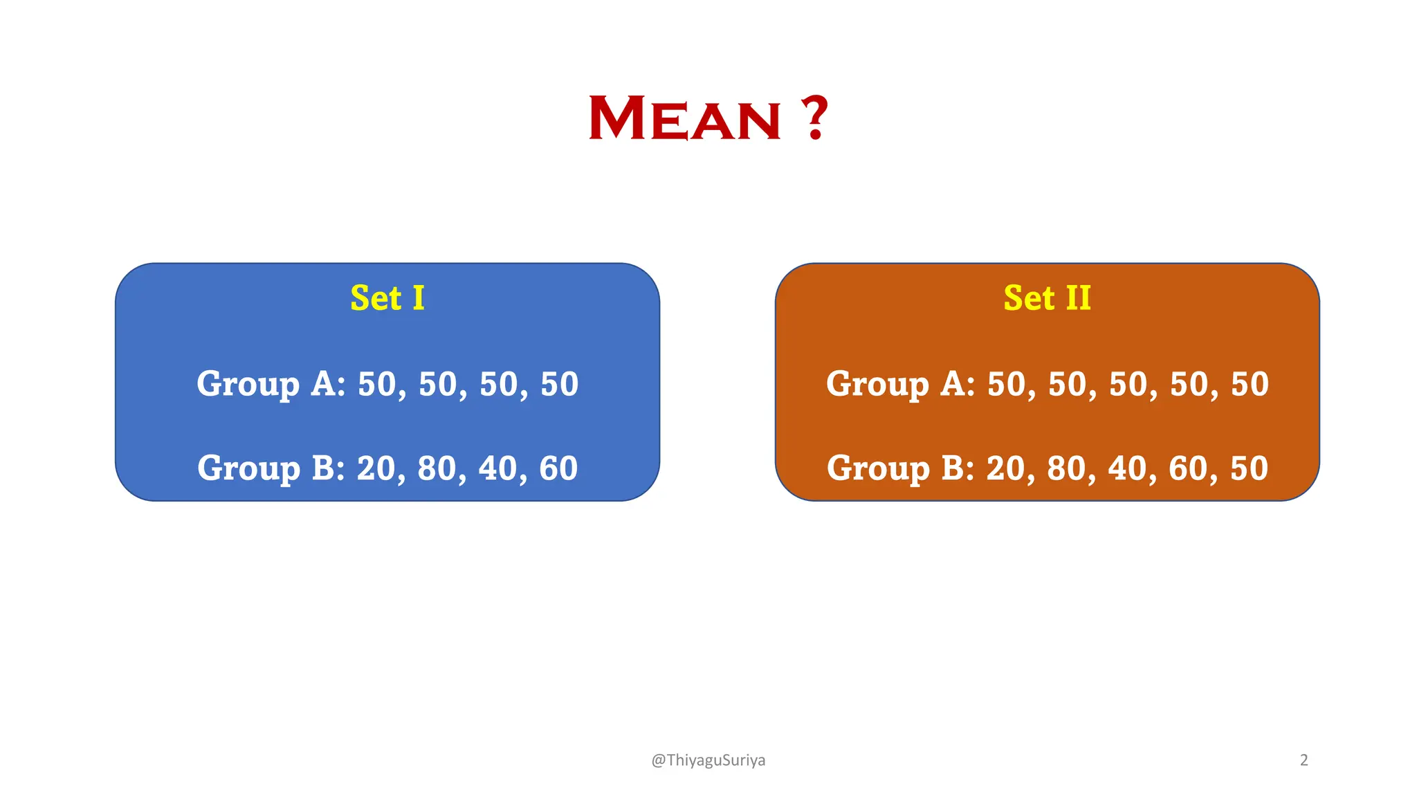
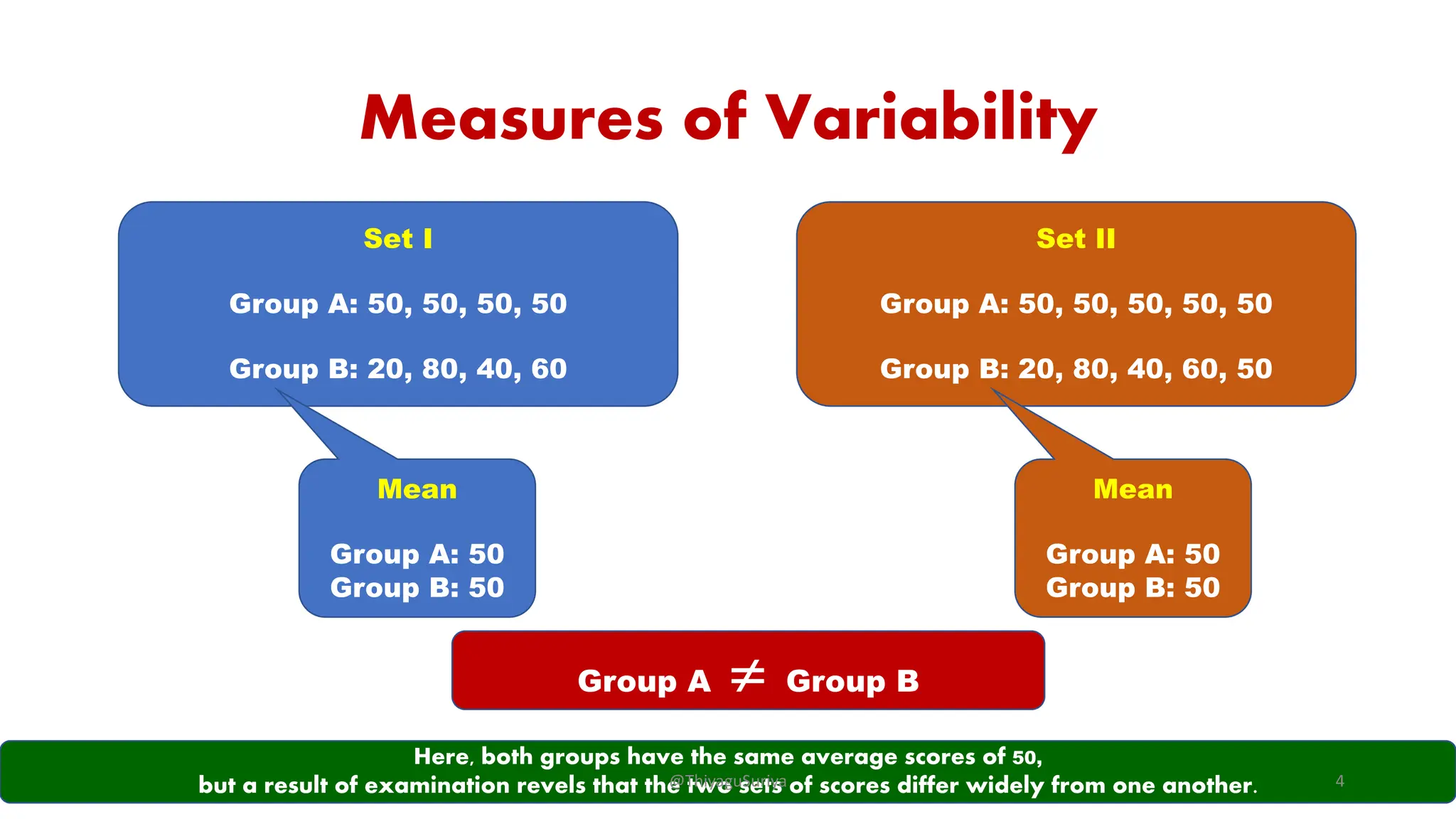
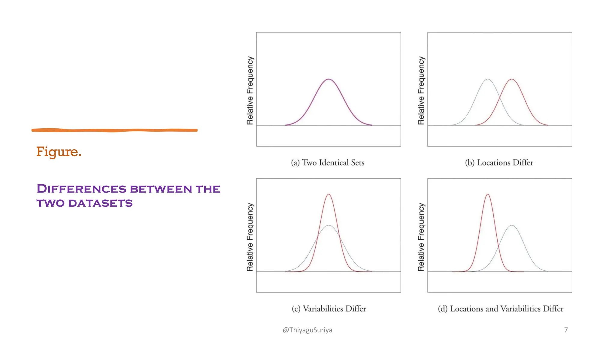
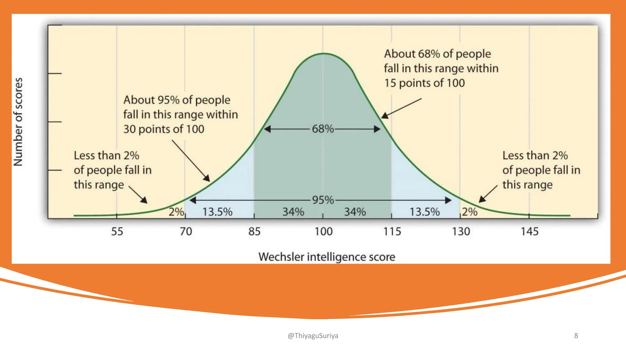
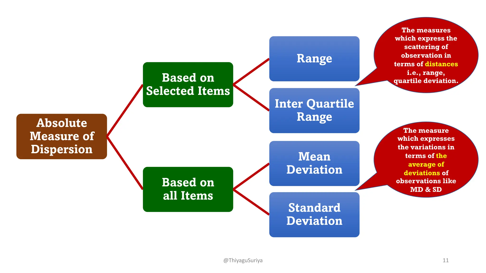
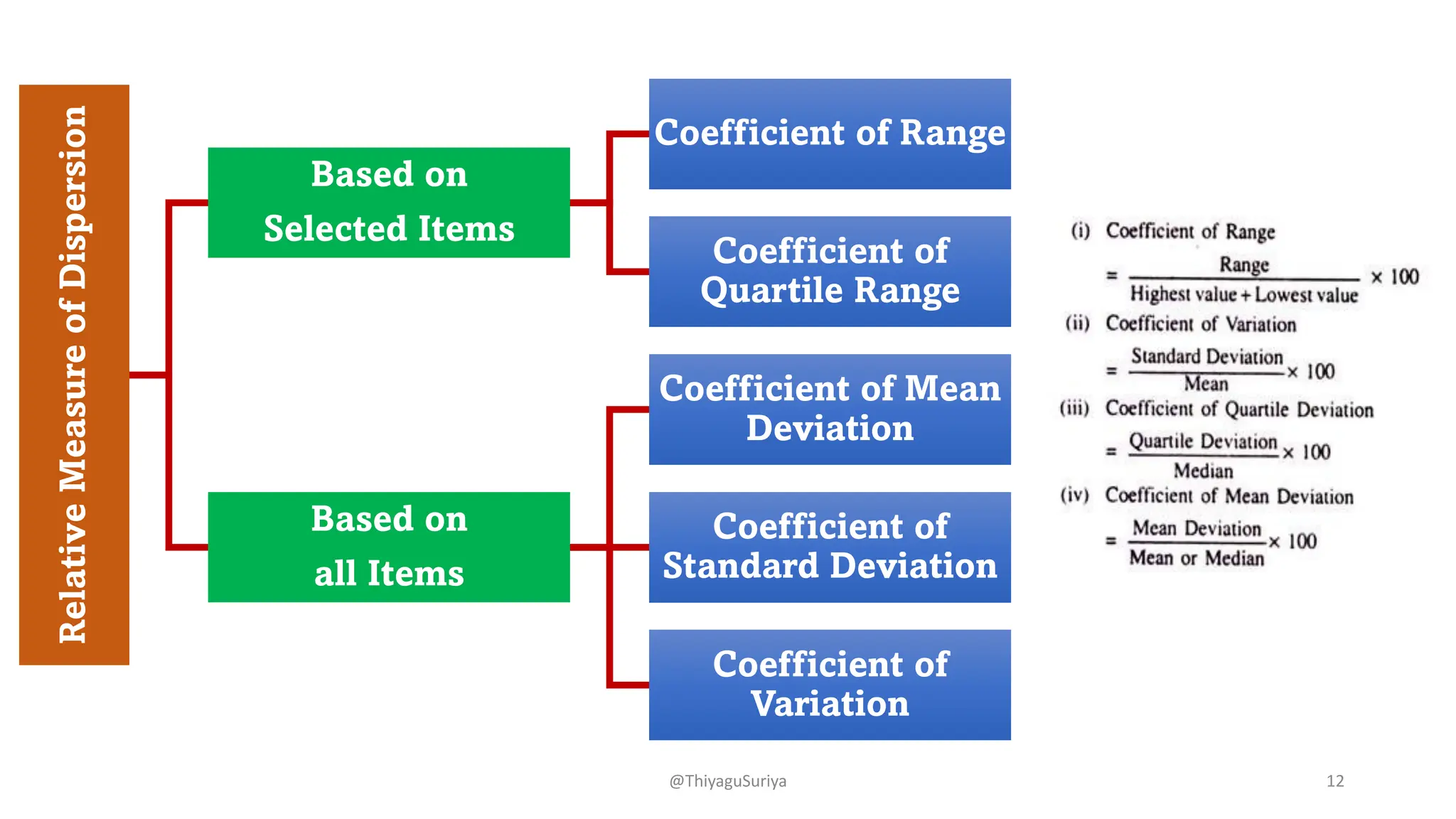
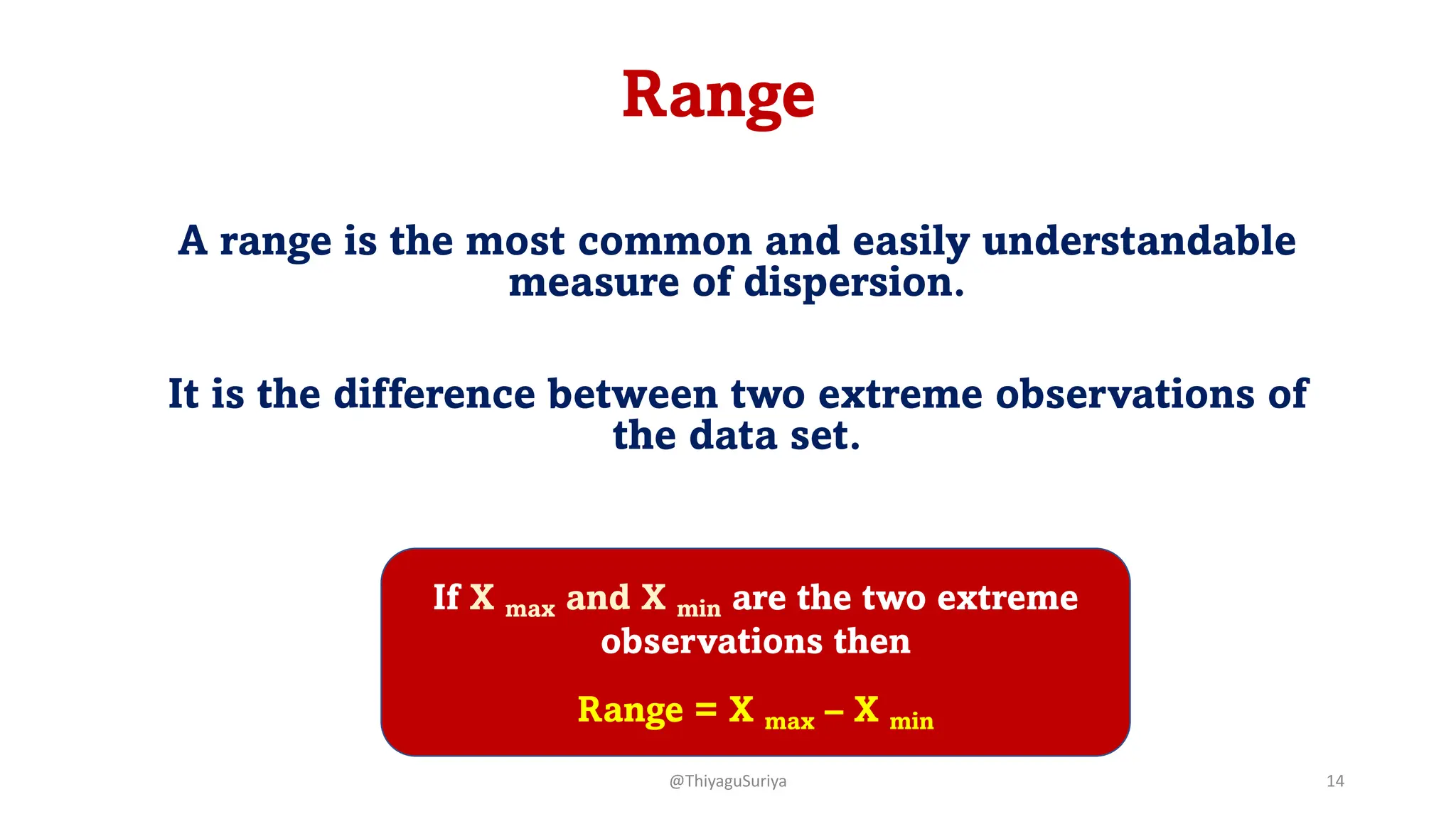
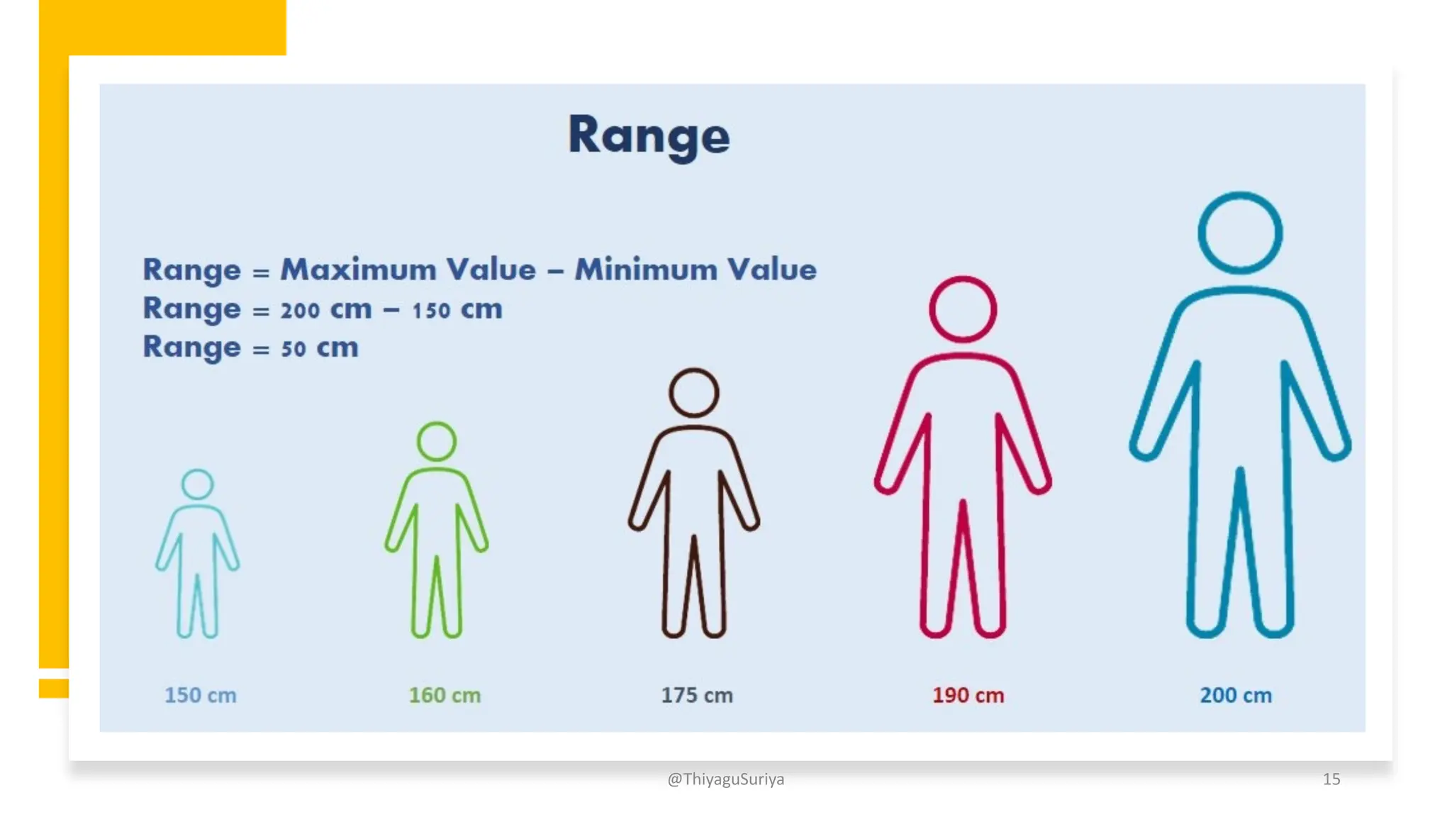
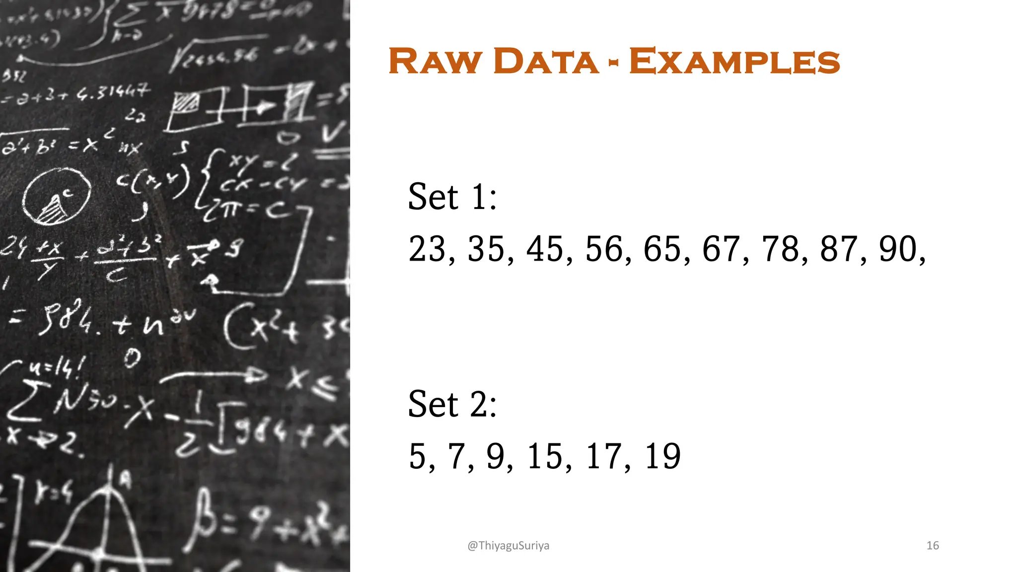
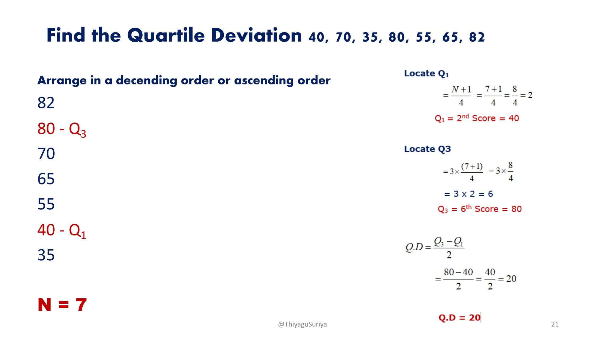
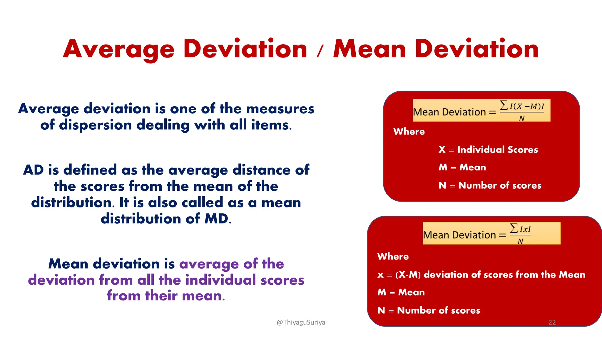
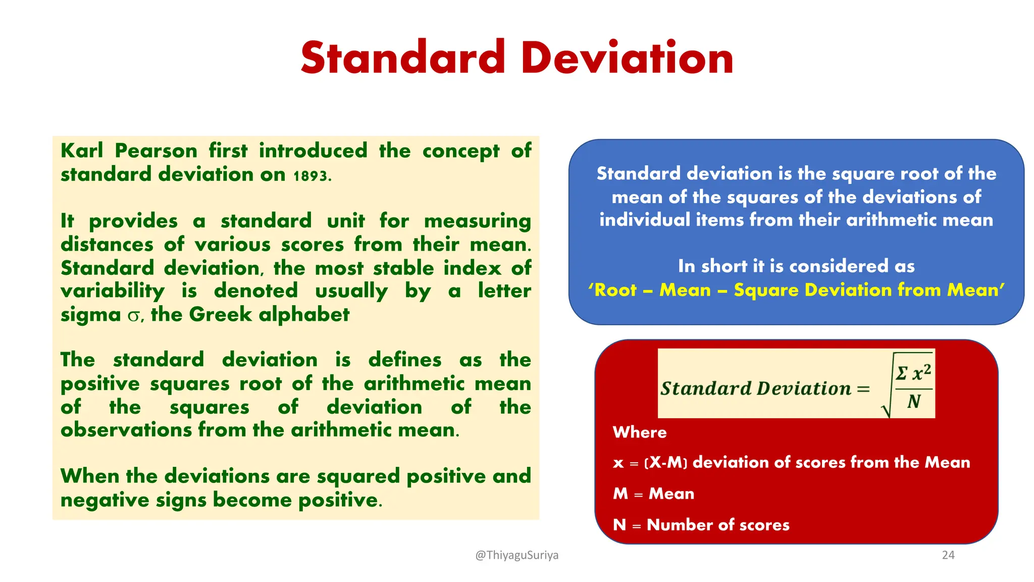
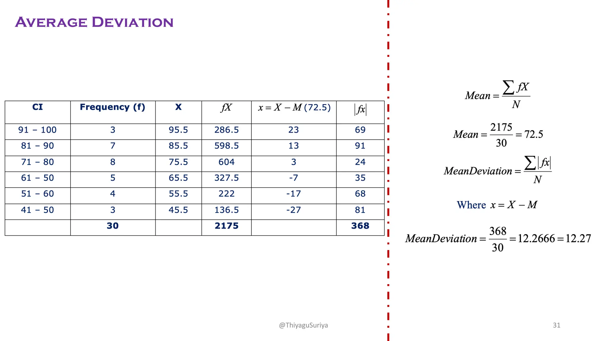
The document discusses measures of dispersion in statistics, highlighting the importance of variability in data interpretation. It explains different methods for calculating dispersion, including range, quartile deviation, mean deviation, and standard deviation. Additionally, it emphasizes the distinction between absolute and relative measures of dispersion and provides examples and formulas for better understanding.

1. Measures
of
Dispersion/
Variability
K.THIYAGU, Assistant
Professor, Department of Education,
Central University of Kerala, Kasaragod @ThiyaguSuriya 1

2. Mean ?
Set I
Group A: 50, 50, 50, 50
Group B: 20, 80, 40, 60
Set II
Group A: 50, 50, 50, 50, 50
Group B: 20, 80, 40, 60, 50
@ThiyaguSuriya 2

3. Mean
Set I
Group A: 50, 50, 50, 50
Group B: 20, 80, 40, 60
Set II
Group A: 50, 50, 50, 50, 50
Group B: 20, 80, 40, 60, 50
Mean
Group A: 50
Group B: 50
Mean
Group A: 50
Group B: 50
Is it means Group A = Group B ?
@ThiyaguSuriya 3

4. Measures of Variability
Set I
Group A: 50, 50, 50, 50
Group B: 20, 80, 40, 60
Set II
Group A: 50, 50, 50, 50, 50
Group B: 20, 80, 40, 60, 50
Mean
Group A: 50
Group B: 50
Mean
Group A: 50
Group B: 50
Group A ¹ Group B
Here, both groups have the same average scores of 50,
but a result of examination revels that the two sets of scores differ widely from one another.
@ThiyaguSuriya 4

5. • Dispersion (also known as
Scatter, Spread or Variation)
is the state of getting
dispersed or spread.
• It measures the degree of
variation.
• Statistical dispersion means
the extent to which numerical
data is likely to vary about an
average value.
Set of data has a small value:
1, 2, 2, 3, 3, 4
…and this set has a wider one:
0, 1, 20, 30, 40, 100
@ThiyaguSuriya 5

6. @ThiyaguSuriya 6

7. Figure.
Differences between the
two datasets
@ThiyaguSuriya 7

8. @ThiyaguSuriya 8

9. Measures of Dispersion
In statistics,
the measures of dispersion
help to interpret the
variability of data
i.e. to know how much
homogenous or heterogenous
the data is.
In simple terms,
it shows
how squeezed or
scattered the variable is.
@ThiyaguSuriya 9

10. Measures
of
Dispersion
Absolute
Measure of
Dispersion
Relative
Measure of
Dispersion
@ThiyaguSuriya 10

11. Absolute
Measure of
Dispersion
Based on
Selected Items
Range
Inter Quartile
Range
Based on
all Items
Mean
Deviation
Standard
Deviation
The measures
which express the
scattering of
observation in
terms of distances
i.e., range,
quartile deviation.
The measure
which expresses
the variations in
terms of the
average of
deviations of
observations like
MD & SD
@ThiyaguSuriya 11

12. Relative
Measure
of
Dispersion
Based on
Selected Items
Coefficient of Range
Coefficient of
Quartile Range
Based on
all Items
Coefficient of Mean
Deviation
Coefficient of
Standard Deviation
Coefficient of
Variation
@ThiyaguSuriya 12

13. C.D. in terms of Coefficient of dispersion
Range C.D. = (Xmax – Xmin) ⁄ (Xmax + Xmin)
Quartile Deviation C.D. = (Q3 – Q1) ⁄ (Q3 + Q1)
Standard Deviation (S.D.) C.D. = S.D. ⁄ Mean
Mean Deviation C.D. = Mean deviation/Average
@ThiyaguSuriya 13

14. Range
A range is the most common and easily understandable
measure of dispersion.
It is the difference between two extreme observations of
the data set.
If X max and X min are the two extreme
observations then
Range = X max – X min
@ThiyaguSuriya 14

15. @ThiyaguSuriya 15

16. Raw Data - Examples
Set 1:
23, 35, 45, 56, 65, 67, 78, 87, 90,
Set 2:
5, 7, 9, 15, 17, 19
@ThiyaguSuriya 16

17. Raw Data - Examples
Set 1:
23, 35, 45, 56, 65, 67, 78, 87, 90,
Range =90 - 23 = 67
Set 2:
5, 7, 9, 15, 17, 19
Range = 19 - 5 = 14
@ThiyaguSuriya 17

18. Quartile Deviation
The quartiles divide a data set into quarters.
The first quartile, (Q1) is the middle number between the
smallest number and the median of the data.
The second quartile, (Q2) is the median of the data set.
The third quartile, (Q3) is the middle number between
the median and the largest number.
Quartile deviation or
semi-inter-quartile deviation is
Q = ½ × (Q3 – Q1)
@ThiyaguSuriya 18

19. ( ) score
N
Q
th
÷
ø
ö
ç
è
æ +
=
4
1
3
3
score
N
Q
mdn
th
÷
ø
ö
ç
è
æ +
=
2
1
)
( 2
score
N
Q
th
÷
ø
ö
ç
è
æ +
=
4
1
1
The value of Q3 can be obtained by the formula
Calculating median we use the formula
The value of Q1 can be obtained by the formula
2
1
3 Q
Q -
QD =
Quartile Deviation from the ungrouped data Formula
@ThiyaguSuriya 19

20. @ThiyaguSuriya 20

21. Find the Quartile Deviation 40, 70, 35, 80, 55, 65, 82
Arrange in a decending order or ascending order
82
80 - Q3
70
65
55
40 - Q1
35
N = 7
@ThiyaguSuriya 21

22. Average Deviation / Mean Deviation
Average deviation is one of the measures
of dispersion dealing with all items.
AD is defined as the average distance of
the scores from the mean of the
distribution. It is also called as a mean
distribution of MD.
Mean deviation is average of the
deviation from all the individual scores
from their mean.
Where
X = Individual Scores
M = Mean
N = Number of scores
Where
x = (X-M) deviation of scores from the Mean
M = Mean
N = Number of scores
@ThiyaguSuriya 22

23. Scores Deviation (Raw Score – Mean) x IxI
10 10 – 30 -20 20
20 20 - 30 -10 10
30 30 – 30 0 0
40 40 – 30 10 10
50 50 - 30 20 20
∑X = 150 ∑IxI = 60
Raw Data: Example:
Calculate A.D. from the following Scores: 10, 20, 30, 40, 50
Where
x = (X-M) deviation of scores from the Mean
M = Mean
N = Number of scores
18 30 42
12 12
M
@ThiyaguSuriya 23

24. Standard Deviation
Karl Pearson first introduced the concept of
standard deviation on 1893.
It provides a standard unit for measuring
distances of various scores from their mean.
Standard deviation, the most stable index of
variability is denoted usually by a letter
sigma s, the Greek alphabet
The standard deviation is defines as the
positive squares root of the arithmetic mean
of the squares of deviation of the
observations from the arithmetic mean.
When the deviations are squared positive and
negative signs become positive.
Standard deviation is the square root of the
mean of the squares of the deviations of
individual items from their arithmetic mean
In short it is considered as
‘Root – Mean – Square Deviation from Mean’
Where
x = (X-M) deviation of scores from the Mean
M = Mean
N = Number of scores
@ThiyaguSuriya 24

25. @ThiyaguSuriya 25

26. Raw Data Examples:
Find out SD of the following scores: 10, 20, 30, 40, 50, 60, 70
Scores7 Deviation (Raw Score – Mean)
x x2
10 10 – 40 -30 900
20 20 - 40 -20 400
30 30 – 40 -10 100
40 40 – 40 0 0
50 50 - 40 10 100
60 60 – 40 20 400
70 70 - 40 30 900
∑X = 280 2800
Where
x = (X-M) deviation of scores from the Mean
M = Mean
N = Number of scores
20 40 60
20 20
M
@ThiyaguSuriya 26

27. Group Data
Measures of Dispersion
@ThiyaguSuriya 27

28. Range
@ThiyaguSuriya 28

29. Class Internal Frequency
91 – 100 3
81 – 90 7
71 – 80 8
61 – 50 5
51 – 60 4
41 – 50 3
Highest Score = 100
Lowest Score = 41
Range = 100 – 41 = 59
Range
@ThiyaguSuriya 29

30. Mean
Deviation
@ThiyaguSuriya 30

31. Average Deviation
@ThiyaguSuriya 31

32. Standard
Deviation
@ThiyaguSuriya 32

33. Standard Deviation
@ThiyaguSuriya 33

34. Quartile
Deviation
@ThiyaguSuriya 34

35. Quartile Deviation
@ThiyaguSuriya 35

36. Quartile Deviation
@ThiyaguSuriya 36

37. Thank You
@ThiyaguSuriya 37

38. Thank
You
@ThiyaguSuriya 38