Measures of Dispersion in business statistics

1. Measures of
Dispersion
DR. DURBA CHAKRABARTY
ITM BUSINESS SCHOOL

2. Why study Dispersion?
► An average, such as the mean or the median only locates the centre of
the data.
► An average does not tell us anything about the spread of the data.
► A small value for a measure of dispersion indicates that the data
are clustered closely (the mean is therefore representative of the
data).
► A large measure of dispersion indicates that the mean is not
reliable (it is not representative of the data).

3. Measures of Dispersion
► Dispersion also known as scatter, spread or variation
► Measures the degree of variation in a set of data
► Measures of dispersion indicate the extent to which the observed values are
“spread out” around that center and how “far apart” observed values typically
are from each other and therefore from some average value (in particular, the
mean)
► For example, in choosing supplier A or supplier B we might consider not
only the average delivery time for each, but also the variability in delivery
time for each.

4. Measures of Dispersion
► Measures of dispersion are descriptive statistics that describe how similar a
set of scores are to each other
► The more similar the scores are to each other, the lower the measure of dispersion will be
► The less similar the scores are to each other, the higher the measure of dispersion will be
► In general, the more spread out a distribution is, the larger the measure of dispersion will
be

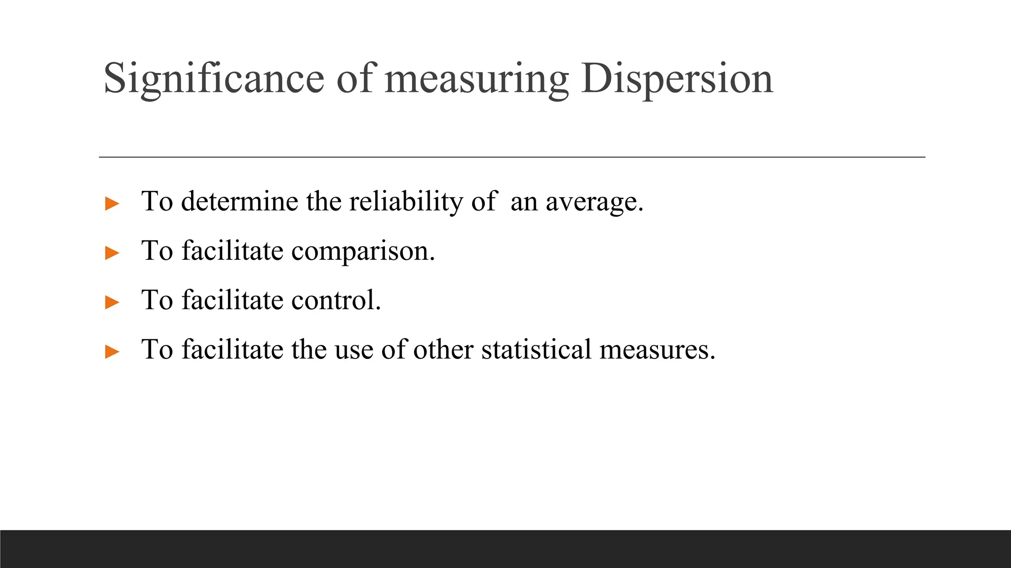
5. Significance of measuring Dispersion
► To determine the reliability of an average.
► To facilitate comparison.
► To facilitate control.
► To facilitate the use of other statistical measures.

6. Absolute Measure
of Dispersion
Based on all items
Based on selected
items
1.Range
2.Inter Quartile Range
1.Mean Deviation
2.Standard Deviation

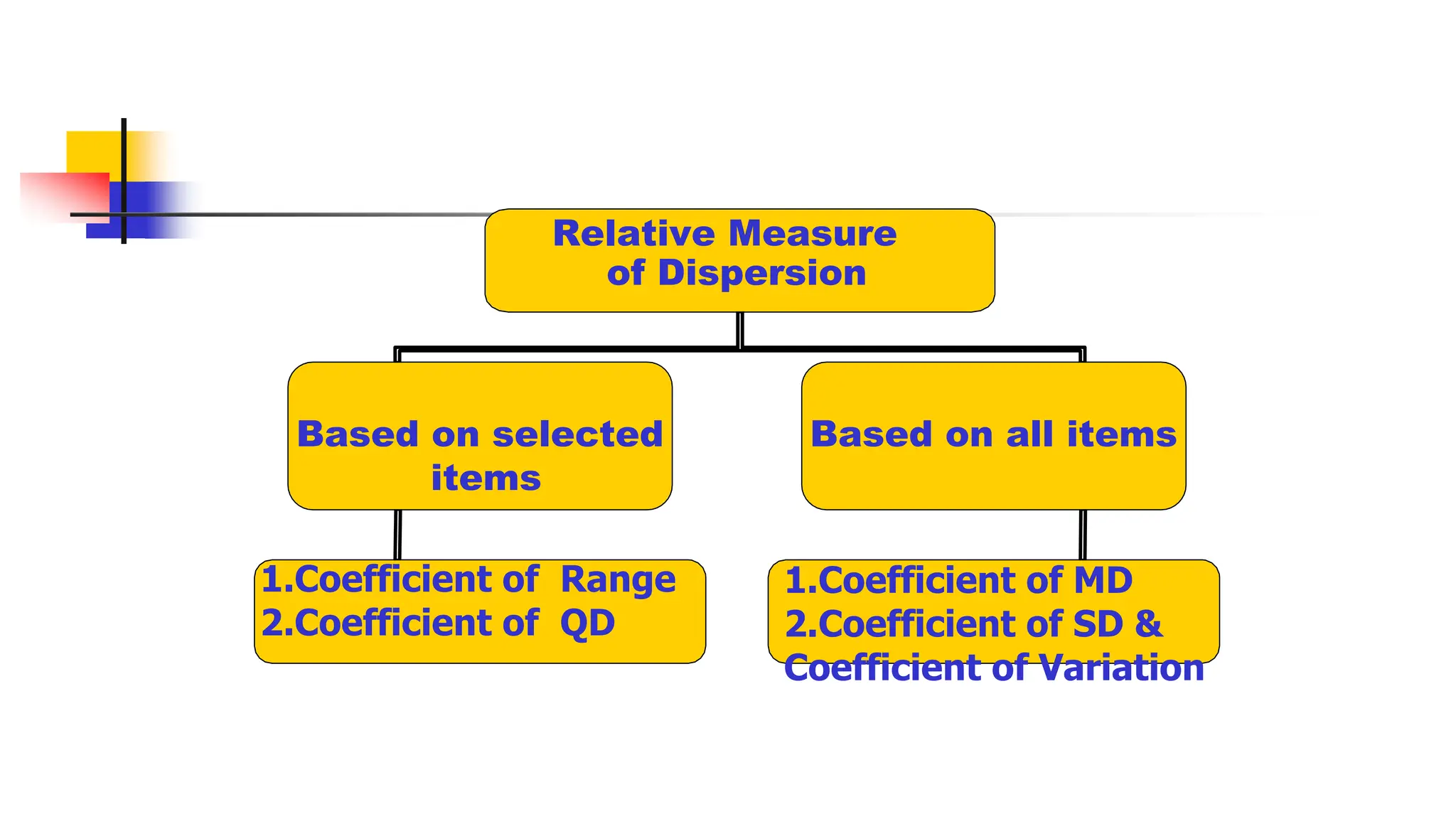
7. Relative Measure
of Dispersion
Based on all items
Based on selected
items
1.Coefficient of Range
2.Coefficient of QD
1.Coefficient of MD
2.Coefficient of SD &
Coefficient of Variation

8. Measures of Variability
► Range
► Interquartile Range
► Variance
► Standard Deviation
► Mean Deviation
► Coefficient of Variation

9. Range
► It is the simplest measure of variability.
► It is easy to compute and to understand. Only two values are used in its calculation
► The range of a data set is the difference between the largest and smallest data
values.
► Range = Largest value – Smallest value
► It is very sensitive to the smallest and largest data values.
► It is influenced by extreme values
► It is used when we have ordinal data

10. Range
Range = largest value - smallest value
Range = 715 - 525 = 190
• Example: Apartment Rents
525 530 530 535 535 535 535 535 540 540
540 540 540 545 545 545 545 545 550 550
550 550 550 550 550 560 560 560 565 565
565 570 570 572 575 575 575 580 580 580
580 585 590 590 590 600 600 600 600 610
610 615 625 625 625 635 649 650 670 670
675 675 680 690 700 700 700 700 715 715

11. Variance

12. • The variance is computed as follows:
• The variance is the average of the squared differences between
each data value and the mean.
for a sample for a population
Variance

13. Standard Deviation
► The standard deviation of a data set is the positive square root of the
variance.
► It is measured in the same units as the data, making it more easily
interpreted than the variance.

14. • The standard deviation is computed as follows:
for a sample for a population
Standard Deviation

15. • The coefficient of variation is computed as follows:
Coefficient of Variation
• The coefficient of variation indicates how large the standard
deviation is in relation to the mean.
for a
sample
for a
population

16. • Variance
• Standard Deviation
• Coefficient of Variation
Sample Variance, Standard Deviation,
And Coefficient of Variation
• Example: Apartment Rents

17. Mean Absolute Deviation
► Mean Absolute Deviation is the average distance between each piece of data
and the mean.
► Measures of variation describe how data values vary by using a single
number
► Steps to find the Mean Absolute Deviation
► Find the mean
► Find the distance between each piece of data and the mean. Remember distance is not
negative so take the absolute value of the difference.
► Find the average of the differences

18. 18
EXAMPLE – Mean Absolute Deviation
The number of cappuccinos sold at the Starbucks location in the Orange Country Airport
between 4 and 7 p.m. for a sample of 5 days last year were 20, 40, 50, 60, and 80.
Determine the mean deviation for the number of cappuccinos sold.

19. Example 1
► Find the mean absolute deviation of the daily visitors to the local
park for one week.
► 234, 540, 502, 629, 530, 450, 574

20. Example 1
► Find the average. 494.1
► Find the distance each piece of data is from the average.
► 260.1, 45.9, 7.9, 134.9, 35.9, 44.1, 79.9
► Find the average of the differences. MD is 87
► The mean number of visitors to the park is 494 visitors per day.
► The MD is 87 which means the average distance from each piece of data is
87 visitors above or below the mean. This shows the spread of the data. The
MD is a higher number because of 234 which is an outlier.

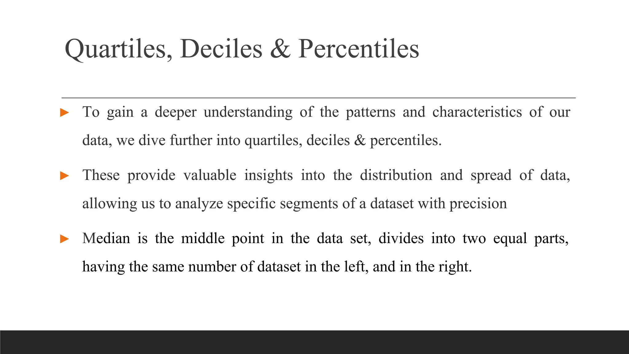
21. Quartiles, Deciles & Percentiles
► To gain a deeper understanding of the patterns and characteristics of our
data, we dive further into quartiles, deciles & percentiles.
► These provide valuable insights into the distribution and spread of data,
allowing us to analyze specific segments of a dataset with precision
► Median is the middle point in the data set, divides into two equal parts,
having the same number of dataset in the left, and in the right.

22. Quartiles, Deciles & Percentiles
► The values which divide an array (a set of data arranged in ascending or
descending order) into four equal parts are called Quartiles.
► The values which divide an array into ten equal parts are called deciles.
► The values which divide an array into one hundred equal parts are called
percentiles.

23. Interquartile Range (IQR)
► The interquartile range of a data set is the difference
between the third quartile and the first quartile.
► It is the range for the middle 50% of the data.
► It overcomes the sensitivity to extreme data values.

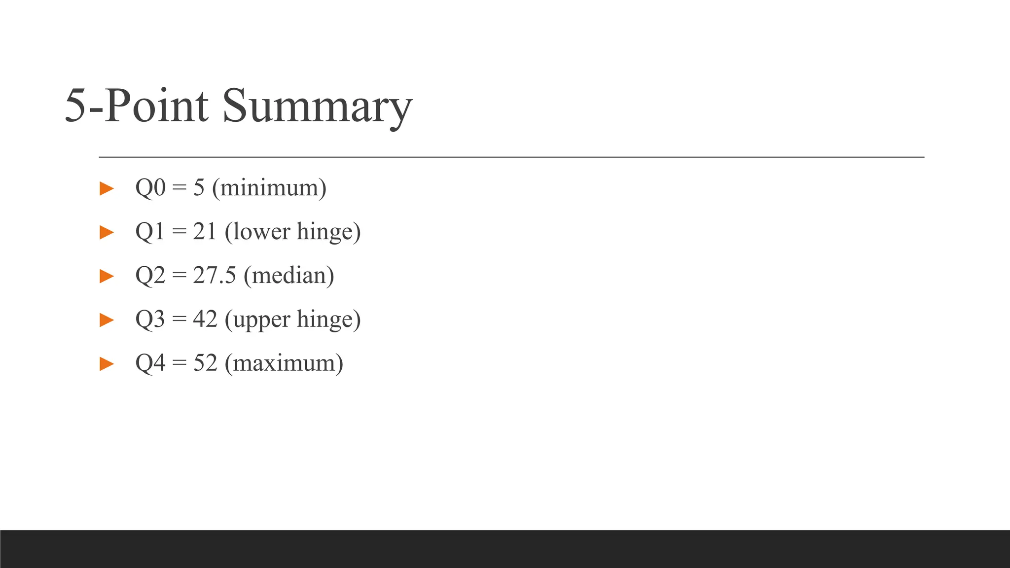
24. Quartiles and IQR
► Quartiles divide the ordered data into four equally-sized groups
► Q0
= minimum
► Q1
= 25th
%ile
► Q2
= 50th
%ile (Median)
► Q3
= 75th
%ile
► Q4
= maximum

25. Illustrative example
► Following is the data of wage rates of workers earned in dollars
► 1362 1439 1460 1614 1666 1792 1867

26. Steps to be followed
► Arrange the data in ascending order
► 1362 1439 1460 1614 1666 1792 1867
► Find the middlemost observation, that is the median.
► In this case it is 1614, that is Q2.
► Next, we consider the Bottom half of data (as median divides the data into two equal parts)
► 1362 1439 1460 1614
► Q1 = (1439 + 1460) / 2 = 1449.5
► Then the Top half of data
► 1614 1666 1792 1867
► Q3 = (1666 + 1792) / 2 = 1729
► 5-point summary: 1362, 1449.5, 1614, 1729, 1867
► IQR= (1729-1449.5)=279.5

27. Rule for quartiles
► Find the median
► Middle of lower half of data set ⇒ Q1
► Middle of upper half of the data ⇒ Q3
Bottom half | Top half
05 11 21 24 27 | 28 30 42 50 52
↑ ↑ ↑
Q1 Q2 Q3
IQR = Q3 – Q1 = 42 – 21 = 21
gives spread of middle 50% of the data

28. 5-Point Summary
► Q0 = 5 (minimum)
► Q1 = 21 (lower hinge)
► Q2 = 27.5 (median)
► Q3 = 42 (upper hinge)
► Q4 = 52 (maximum)

29. Which Measure of Dispersion to go
ahead?
▪Standard deviation (or variance) is usually preferable.
▪However, the standard deviation (or variance) isn’t appropriate when there are
extreme scores and/or skewness in your data set. In this situation the interquartile
range is usually preferable.
▪Standard Deviation is used as a measure of dispersion when mean is used as
measure of central tendency (i.e., for symmetric numerical data).
▪For ordinal data or skewed numerical data, median and interquartile range are
used.