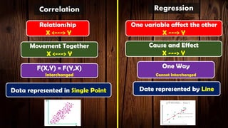
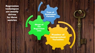
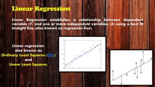
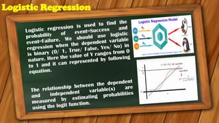
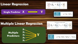
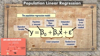
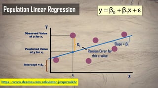
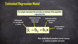
The document provides an overview of various regression analysis techniques used in statistical modeling, including linear, logistic, polynomial, stepwise, ridge, lasso, and elastic-net regression. It outlines their purposes, how they handle different types of data, and describes the assumptions and tests necessary for each method. Additionally, it discusses the historical background of regression and its applications in predicting dependent variables based on independent variables.

1. Regression
Analysis
K.THIYAGU,
Assistant Professor,
Department of Education,
Central University of Kerala, Kasaragod

3. Correlation Regression
X
Y

4. Correlation Regression
Relationship
X <---> Y
One variable affect the other
X ---> Y
Movement Together
X <---> Y
Cause and Effect
X ---> Y
F(X,Y) = F(Y,X)
Interchanged
One Way
Cannot Interchanged
Data represented in Single Point Date represented by Line

5. Number of
Independent
Variables
Shape of
the
Regression
Line
Type of
Dependent
Variable
Regression
techniques
are mostly
driven
by three
metrics

6. Linear Regression
Linear Regression establishes a relationship between dependent
variable (Y) and one or more independent variables (X) using a best fit
straight line (also known as regression line).
Linear regression,
also known as
Ordinary Least Squares (OLS)
and
Linear Least Squares.

7. Logistic Regression

8. Polynomial Regression
In this regression technique, the best fit line
is not a straight line. It is rather a curve that
fits into the data points.
Polynomial regression is similar to multiple
linear regression. However, in this type of
regression the relationship between X and Y
variables is defined by taking the k-th degree
polynomial in X.
y=a+b*x^2

9. Stepwise Regression
This form of regression is used when we deal
with multiple independent variables.
In this technique, the selection of independent
variables is done with the help of an automatic
process, which involves no human intervention.

10. Ridge Regression
Ridge Regression is a technique used when the data
suffers from multicollinearity (independent variables
are highly correlated). In multicollinearity, even
though the least squares estimates (OLS) are
unbiased, their variances are large which deviates the
observed value far from the true value. By adding a
degree of bias to the regression estimates, ridge
regression reduces the standard errors.
However, when the predictor variables are highly
correlated (when predictors A and B change in a
similar manner) small amount of bias factor is
included to alleviate the problem.

11. Lasso Regression
LASSO (Least Absolute Shrinkage Selector Operator) is
another alternative to Ridge regression but the only
difference is that it penalizes the absolute size of the
regression coefficients. By penalizing the absolute
values, the estimated coefficients shrink more towards
zero which could not be possible using ridge regression.
This method makes it useful for feature selection where
a set or variables and parameters are picked for model
construction. LASSO takes the relevant features and
zeroes the irrelevant values such that overfitting is
avoided and also makes the learning faster. Hence,
LASSO is both a feature selection model and a
regularization model.

12. ElasticNet
Regression
ElasticNet is a hybrid to both
LASSO and Ridge regression
which combines the linear L1
and L2 penalties of the two and
is preferred over the two
methods for many applications.
Elastic-net is useful when there
are multiple features which are
correlated. Lasso is likely to pick
one of these at random, while
elastic-net is likely to pick both.

13. Regression
Independent Variable(s) Dependent Variable
Count(s) Scale Count Scale
Simple
Linear
1 Interval or Ratio 1 Interval or Ratio
Multiple
Linear regression
2+ Interval or Ratio
or Dichotomous
1 Interval or Ratio
Logistic
regression
2+ Interval or Ratio
or Dichotomous
1 Dichotomous
Ordinal
regression
1+ Nominal or
Dichotomous
1 Ordinal
Multinomial
regression
1+ Interval or Ratio
or Dichotomous
1 Nominal
Discriminant
Analysis
1+ Interval or Ratio 1 Nominal

14. • It was introduced by Sir Francis
Galton in 1877 in his study of
heredity.
• The term regression has been
derived from the word ‘to
regress’ which means tendency
to go back.
• This statistical method is
employed for predicting or
estimating the unknown value
called dependent variable,
from value of another variable
is known as independent
variable.

15. •Predictor or
•Independent Variable (IV)
X
•Criterion or
•Dependent Variable (DV)
Y
Use scores on one variable X
to predict scores on another variable Y.
Simple Regression

16. Linear Regression
Single Predictor X Y
Multiple Linear Regression
X1
X2
X3
X4
X5
Y
Multiple
Predictors

17. εxββy 10 ++=
Linear component
Population Linear Regression
The population regression model:
Population
y intercept
Population
Slope
Coefficient
Random
Error
term, or
residualDependent
Variable
Independent
Variable
Random Error
component

18. Population Linear Regression
Random Error for
this x value
y
x
Observed Value
of y for xi
Predicted Value
of y for xi
εxββy 10 ++=
xi
Slope = β1
Intercept = β0
εi
https://www.desmos.com/calculator/jwquvmikhr

19. xbbyˆ 10i +=
The sample regression line provides an estimate of the population
regression line
Estimated Regression Model
Estimate of the
regression
intercept
Estimate of the
regression
slope
Estimated
(or predicted)
y value
Independent
variable
The individual random error terms
ei have a mean of zero

20. Regression Equation
Average value of ‘y’ is a function of ‘x’
Y = a*x + b

21. Simple
Linear
Regression

22. IV = 1
DV = 1
Simple
Regression
IVs=2+
DV = 1
Multiple
Regression

23. • Two variables should be measured at the continuous
level (Interval or Ratio)Assumption # 1
• Linear relationship between two variables
Assumption # 2
• No Significant outliers
Assumption # 3
• Independence of observation (Checked by Durbin
Watson Statistic)Assumption # 4
• Data needs to show homoscedasticity
Assumption # 5
• Residuals of the regression line are approximately
normally distributedAssumption # 6

24. Linear Vs NonLinear (Curvilinear)

25. Vs
Heteroscedasticity Homoscedasticity

26. Outlier

27. Residual

28. Important Values
in Regression
Assumption Tests Scores
Outliers Standard Residual Not exceed  3.29
Independence Observation Durbin Watson Not exceed -1 to +3
Multicollinearity Tolerance Should be 0.10 or greater
Multicollinearity VFI Not Greater that 10

29. SPSS Path
Analyse Regression Linear

30. Beta – the standardized coefficient value is equal to the Pearson correlation
coefficient value between the two variables in simple regression.

31. Model Summary Table – Output
• Multiple Correlation Coefficient; in simple
regression is it equal to the Pearson correlationR
• The amount of variance in the DV (criterion) that is
accounted for or explained by the IV (predictor)
• (IV explains …percentage of the variance in DV)
R2

32. Df= N-2, where N = the number of pairs of scores

33. Relationship between F and t
(Simple Regression)
F t2

34. MULTIPLE REGRESSION
{2+ Predictors (Ivs)}

35. Hierarchical Regression
{2+ Predictors (With order of Model)}
If a predictor accounts for a significant amount of unique variance above
and beyond one or more predictors that have already been entered into
the model.

36. •A procedure for variable selection in which all variables in a block
are entered in a single step.Enter
• At each step, the independent variable not in the equation that has the
smallest probability of F is entered, if that probability is sufficiently small.
Variables already in the regression equation are removed if their
probability of F becomes sufficiently large. The method terminates when no
more variables are eligible for inclusion or removal.
Stepwise.
•A procedure for variable selection in which all variables in a block
are removed in a single step.Remove
•A variable selection procedure in which all variables are entered into the equation and
then sequentially removed. The variable with the smallest partial correlation with the
dependent variable is considered first for removal. If it meets the criterion for
elimination, it is removed. After the first variable is removed, the variable remaining in
the equation with the smallest partial correlation is considered next. The procedure
stops when there are no variables in the equation that satisfy the removal criteria.
Backward
Elimination.
•A stepwise variable selection procedure in which variables are sequentially entered
into the model. The first variable considered for entry into the equation is the one with
the largest positive or negative correlation with the dependent variable. This variable
is entered into the equation only if it satisfies the criterion for entry. If the first variable
is entered, the independent variable not in the equation that has the largest partial
correlation is considered next. The procedure stops when there are no variables that
meet the entry criterion.
Forward
Selection.
Regression Method

37. Thank
you