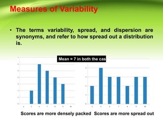
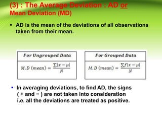
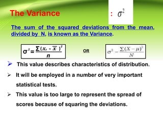
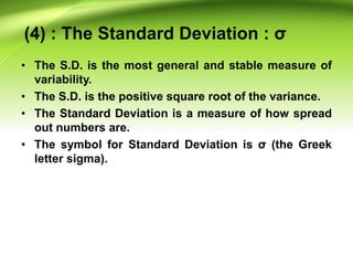
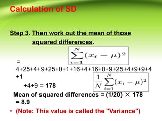
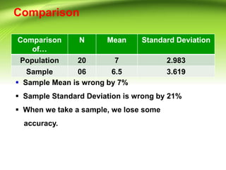
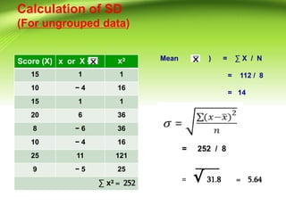
This document discusses various measures of variability that can be used to describe how spread out a distribution is. It describes four major measures: range, quartile deviation, average deviation, and standard deviation. The range is the simplest measure, being the difference between the highest and lowest values. The quartile deviation uses the interquartile range to describe the middle 50% of scores. The average deviation takes the average of all deviations from the mean. The standard deviation is the most common measure, being the positive square root of the variance, which is the average of the squared deviations from the mean. Examples are provided for calculating each measure using both grouped and ungrouped data.


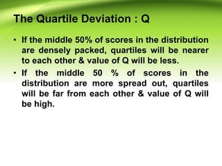

![A Deviation score
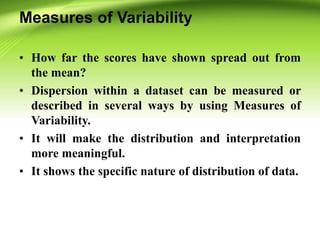
• A score expressed as its distance from the
Mean is called a deviation score.
x = ( X − )
e.g. 6, 5, 4, 3, 2, 1 Mean ( ) = 21/6 = 3.50
[ e.g. 6 – 3.50 = 2.5 is a deviation score of
6 ]
Sum of deviations of each value from the
mean :
2.5 + 1.5 + 0.5 + (- 0.5) + (- 1.5 ) + (- 2.5 ) = 0
) = 0 ∑ x = 0](https://image.slidesharecdn.com/measureofvariabilitywindri-240223113333-6faace5e/85/measure-of-variability-windri-In-research-include-example-16-320.jpg)

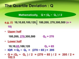
![The Standard Deviation : Formulas
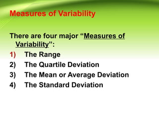
• The Population Standard Deviation:
•
• The Sample Standard Deviation:
• The important change is "N-1" instead of
"N" (which is called "Bessel's correction”-
Friedrich Bessel ).
• [ The factor n/(n − 1) is itself called Bessel's correction.]](https://image.slidesharecdn.com/measureofvariabilitywindri-240223113333-6faace5e/85/measure-of-variability-windri-In-research-include-example-24-320.jpg)


![[DSC Europe 25] Josip Saban - Career building for data professionals.pptx](https://cdn.slidesharecdn.com/ss_thumbnails/zroflcttkm1vmli0txea-josip-saban-career-building-for-data-professionals-260123083019-587cdb8c-thumbnail.jpg?width=640&height=640&fit=bounds)