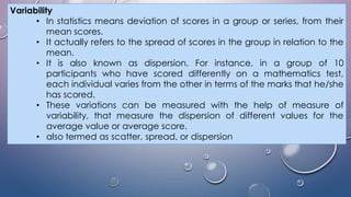
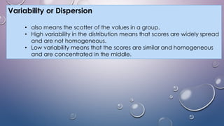
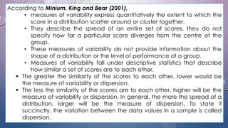
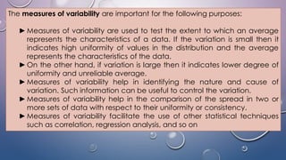
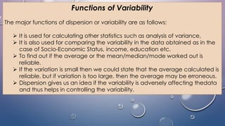
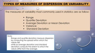
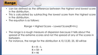
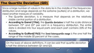
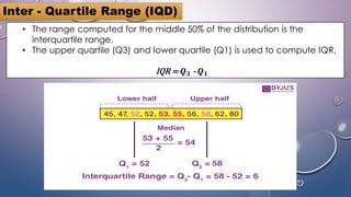
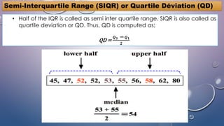
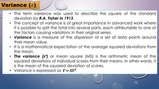
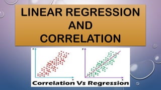
The document discusses various concepts related to variability and measures of dispersion in statistics: - Variability refers to the spread or deviation of scores from the mean in a data set. Measures of variability quantify how concentrated or dispersed the data is. - Common measures of variability include range, quartile deviation, mean deviation, variance, standard deviation, and coefficient of variation. Range simply measures the highest and lowest scores while other measures account for dispersion across all scores. 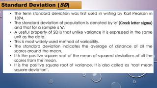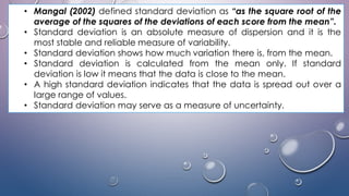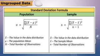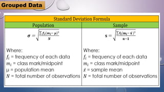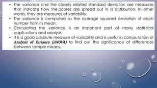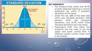- The standard deviation is the most widely used measure of variability as it expresses dispersion in the same units as the original data. It quantifies how far scores deviate from the mean on average. - Understanding variability is important for determining if averages

1. MEASURE
OF
VARIABILITY

2. Variability
• In statistics means deviation of scores in a group or series, from their
mean scores.
• It actually refers to the spread of scores in the group in relation to the
mean.
• It is also known as dispersion. For instance, in a group of 10
participants who have scored differently on a mathematics test,
each individual varies from the other in terms of the marks that he/she
has scored.
• These variations can be measured with the help of measure of
variability, that measure the dispersion of different values for the
average value or average score.
• also termed as scatter, spread, or dispersion

3. Variability or Dispersion
• also means the scatter of the values in a group.
• High variability in the distribution means that scores are widely spread
and are not homogeneous.
• Low variability means that the scores are similar and homogeneous
and are concentrated in the middle.

4. According to Minium, King and Bear (2001),
• measures of variability express quantitatively the extent to which the
score in a distribution scatter around or cluster together.
• They describe the spread of an entire set of scores, they do not
specify how far a particular score diverges from the centre of the
group.
• These measures of variability do not provide information about the
shape of a distribution or the level of performance of a group.
• Measures of variability fall under descriptive statistics that describe
how similar a set of scores are to each other.
 The greater the similarity of the scores to each other, lower would be
the measure of variability or dispersion.
 The less the similarity of the scores are to each other, higher will be the
measure of variability or dispersion. In general, the more the spread of a
distribution, larger will be the measure of dispersion. To state it
succinctly, the variation between the data values in a sample is called
dispersion.

5. Variability or Dispersion
• is also known as the average of the second degree, because here we
consider the arithmetic mean of the deviations from the mean of the
values of the individual items. To describe a distribution adequately,
therefore, we usually must provide a measure of central tendency and a
measure of variability. Measures of variability are important in statistical
inference.
• With the help of measures of dispersion, we can know about fluctuation
in random sampling. How much fluctuation will occur in random
sampling?
• This question in fundamental to every problem in statistical inference, it is
a question about variability.

6. The measures of variability are important for the following purposes:
►Measures of variability are used to test the extent to which an average
represents the characteristics of a data. If the variation is small then it
indicates high uniformity of values in the distribution and the average
represents the characteristics of the data.
►On the other hand, if variation is large then it indicates lower degree of
uniformity and unreliable average.
►Measures of variability help in identifying the nature and cause of
variation. Such information can be useful to control the variation.
►Measures of variability help in the comparison of the spread in two or
more sets of data with respect to their uniformity or consistency.
►Measures of variability facilitate the use of other statistical techniques
such as correlation, regression analysis, and so on

7. Functions of Variability
The major functions of dispersion or variability are as follows:
 It is used for calculating other statistics such as analysis of variance,
 It is also used for comparing the variability in the data obtained as in the
case of Socio-Economic Status, income, education etc.
 To find out if the average or the mean/median/mode worked out is
reliable.
 If the variation is small then we could state that the average calculated is
reliable, but if variation is too large, then the average may be erroneous.
 Dispersion gives us an idea if the variability is adversely affecting thedata
and thus helps in controlling the variability.

8. TYPES OF MEASURES OF DISPERSION OR VARIABILITY
The measures of variability most commonly used in statistics are as follow:
 Range
 Quartile Deviation
 Average Deviation or Mean Deviation
 Variance
 Standard Deviation
Note:
Range and quartile deviation measure dispersion
by computing the spread within which the
values fall,
while as average deviation and standard
deviation compute the extent to which the
values differ from the average.

9. • can be defined as the difference between the highest and lowest score
in the distribution.
• This is calculated by subtracting the lowest score from the highest score
in the distribution.
• The equation is as follows:
Range = Highest Score – Lowest Score(R=H-L)
• The range is a rough measure of dispersion because it tells about the
spread of the extreme scores and not the spread of any of the scores in
between.
• For instance, the range for the distribution 4,10,12,20, 25, 50 will be
R = H – L
R = 50 - 4
R = 46
Range

10. Since a large number of values in the data lie in the middle of the frequencies
distribution and range depends on the extreme (outliers) of a distribution, we
need another measure of variability.
• The Quartile deviation, is a measure that depends on the relatively
stable central portion of a distribution.
• According to Garret (1966), the Quartile deviation is half the scale distance
between 75th and 25th per cent in a frequency distribution. The entire
data is divided into four equal parts and each part contains 25% of the
values.
• According to Guilford(1963) the Semi-Interquartile range is the one half the
range of the middle 50 percent of the cases.
The Quartile Deviation (QD)
On the basis of above definitions, it can be said that quartile deviation
is half the distance between Q1 and Q3.

11. • The range computed for the middle 50% of the distribution is the
interquartile range.
• The upper quartile (Q3) and lower quartile (Q1) is used to compute IQR.
IQR = 𝑸𝟑 - 𝑸𝟏
Inter - Quartile Range (IQD)

12. Semi-Interquartile Range (SIQR) or Quartile Déviation (QD)
• Half of the IQR is called as semi inter quartile range. SIQR is also called as
quartile deviation or QD. Thus, QD is computed as;
QD =
𝑸𝟑 − 𝑸𝟏
𝟐

13. • The term standard deviation was first used in writing by Karl Pearson in
1894.
• The standard deviation of population is denoted by ‘σ’ (Greek letter sigma)
and that for a sample is ‘s’.
• A useful property of SD is that unlike variance it is expressed in the same
unit as the data.
• This is most widely used method of variability.
• The standard deviation indicates the average of distance of all the
scores around the mean.
• It is the positive square root of the mean of squared deviations of all the
scores from the mean.
• It is the positive square root of variance. It is also called as ‘root mean
square deviation’.
Standard Deviation (SD)

14. • Mangal (2002) defined standard deviation as “as the square root of the
average of the squares of the deviations of each score from the mean”.
• Standard deviation is an absolute measure of dispersion and it is the
most stable and reliable measure of variability.
• Standard deviation shows how much variation there is, from the mean.
• Standard deviation is calculated from the mean only. If standard
deviation is low it means that the data is close to the mean.
• A high standard deviation indicates that the data is spread out over a
large range of values.
• Standard deviation may serve as a measure of uncertainty.

15. Ungrouped Data

16. Grouped Data

17. Variance (𝜎)
• The term variance was used to describe the square of the standard
deviation by R.A. Fisher in 1913.
• The concept of variance is of great importance in advanced work where
it is possible to split the total into several parts, each attributable to one of
the factors causing variations in their original series.
• Variance is a measure of the dispersion of a set of data points around
their mean value.
• It is a mathematical expectation of the average squared deviations from
the mean.
• The variance (s²) or mean square (MS) is the arithmetic mean of the
squared deviations of individual scores from their means. In other words, it
is the mean of the squared deviation of scores.
• Variance is expressed as V = SD²

18. • The variance and the closely related standard deviation are measures
that indicate how the scores are spread out in a distribution. In other
words, they are measures of variability.
• The variance is computed as the average squared deviation of each
number from its mean.
• Calculating the variance is an important part of many statistical
applications and analysis.
• It is a good absolute measure of variability and is useful in computation of
Analysis of Variance (ANOVA) to find out the significance of differences
between sample means.

20. Find the variance and
standard deviation of the
following sample data:
1. 5, 17, 12, 10
2.
Example: Solution: #1
𝒙𝒊 𝒙𝒊 - x̄ (𝒙𝒊 - x̄ )²
5 -6 36
10 -1 1
12 1 1
17 6 36
σ (𝐱𝐢 − x̄ )² = 74
𝐬 =
σ(𝒙𝐢− 𝐱 )²
𝐧−𝟏
𝐬 =
𝟕𝟒
𝟑
𝐬 = 4.97
𝐬² =
σ(𝒙𝐢− 𝐱 )²
𝐧−𝟏
𝐬² =
𝟕𝟒
𝟑
𝐬² = 24.67

21. Solution: #2
Class Frequency (𝒇𝒊) 𝒎𝒊 𝒎𝒊 − x̄ (𝒎𝒊 − x̄)² 𝒇𝒊(𝒎𝒊 − x̄)²
40-44 7 42 -13 169
1183
45-49 10 47 -8 64
640
50-54 22 52 -3 9
198
55-59 15 57 2 4
60
60-64 12 62 7 49
588
65-69 6 67 12 144
864
70-74 3 72 17 289
867
σ 𝒇𝒊 = 75 σ 𝒇𝒊(𝒎𝒊 − x̄)²
= 4400
𝐬² =
σ 𝒇𝒊(𝒎𝒊 − x̄)²
𝐧−𝟏
𝐬² =
𝟒𝟒𝟎𝟎
𝟕𝟒
𝐬² = 59.46
𝐬 =
σ(𝒙𝐢− 𝐱 )²
𝐧−𝟏
𝐬 =
𝟒𝟒𝟎𝟎
𝟕𝟒
𝐬 = 7.71

22. Co-efficient of Variation (CV)
The relative measure corresponding to SD is the coefficient of variation.
• It is a relative measure of dispersion developed by Karl Pearson.
• When we want to compare the variations (dispersion) of two different
series, relative measures of standard deviation must be calculated.
• This is known as co-efficient of variation or the co-efficient of SD. It is
defined as the SD expressed as a percentage of the mean.
• The coefficient of variation represents the ratio of the standard
deviation to the mean, and it is a useful statistic for comparing the
degree of variation from one data series to another, even if the
means are drastically different from each other.
• Thus, it is more suitable than SD or variance.
• It is given as a percentage and is used to compare the consistency or
variability of two or more data series.

23. The formula for computing coefficient of variation is as follows:
CV =
σ
𝑴
× 100
Where,
CV = coefficient of variation
σ = Standard deviation
M = Mean
Example:
If the standard deviation of marks obtained by 10 students in a class test in
English is 10 and Mean is 79, then,
CV =
σ
𝑴
× 100
CV =
10
𝟕𝟗
× 100
CV = 12.658

24. • also sometimes called the three-sigma or 68-95-99.7 rule.
• a statistical rule which states that for normally distributed data, almost all
observed data will fall within three standard deviations (denoted by the Greek
letter sigma, or σ) of the mean or average (represented by the Greek letter mu,
or µ) of the data.
• in particular, the empirical rule predicts that in normal distributions, 68% of
observations fall within the first standard deviation (µ ± σ), 95% within the first two
standard deviations (µ ± 2σ), and 99.7% within the first three standard deviations
(µ ± 3σ) of the mean.
• also used as a rough way to test a distribution's "normality." If too many data
points fall outside the three standard deviation boundaries, this suggests that the
distribution is not normal and may be skewed or follow some other distribution.
Empirical Rule

26. KEY TAKEAWAYS
• The Empirical Rule states that 99.7%
of data observed following a normal
distribution lies within 3 standard
deviations of the mean.
• Under this rule, 68% of the data falls
within one standard deviation, 95%
percent within two standard
deviations, and 99.7% within three
standard deviations from the mean.
• Three-sigma limits that follow the
empirical rule are used to set the
upper and lower control limits in
statistical quality control charts and
in risk analysis.

27. Uses of Empirical Rule
• is applied to anticipate probable outcomes in a normal distribution.
• For instance, a statistician would use this to estimate the percentage of cases that fall
in each standard deviation.
• Consider that the standard deviation is 3.1 and the mean equals 10.
In this case,
• the first standard deviation would range between (10+3.2)= 13.2 and (10-3.2)= 6.8.
• The second deviation would fall between 10 + (2 X 3.2)= 16.4
• and 10 - (2 X 3.2)= 3.6, and so forth.
Benefits of the Empirical Rule
• The empirical rule is beneficial because it serves as a means of forecasting data.
• This is especially true when it comes to large datasets and those where variables are
unknown.
• In finance specifically, the empirical rule is germane to stock prices, price indices, and
log values of forex rates, which all tend to fall across a bell curve or normal distribution.

28. • a measure of the asymmetry of a distribution.
• A distribution is asymmetrical when its left and right side are not
mirror images.
• A distribution can have right (or positive), left (or negative), or
zero skewness.
• A right-skewed distribution is longer on the right side of its peak,
and a left-skewed distribution is longer on the left side of its peak:
Skewness

29. What is zero skew?
• When a distribution has zero skew, it is symmetrical. Its left and right sides are mirror
images.
• Normal distributions have zero skew, but they’re not the only distributions with zero skew.
Any symmetrical distribution, such as a uniform distribution or some bimodal (two-peak)
distributions, will also have zero skew.
• The easiest way to check if a variable has a skewed distribution is to plot it in a histogram.
For example, the weights of six-week-old chicks are shown in the histogram below.
• The distribution is approximately symmetrical, with the observations distributed similarly on
the left and right sides of its peak. Therefore, the distribution has approximately zero skew.

30. What is right skew (positive skew)?
• A right-skewed distribution is longer on the right side of its peak than on its
left.
• Right skew is also referred to as positive skew.
• A right-skewed distribution has a long tail on its right side.
• The number of sunspots observed per year, shown in the histogram
below, is an example of a right-skewed distribution.
• The sunspots, which are dark, cooler areas on the surface of the sun,
were observed by astronomers between 1749 and 1983.
• The distribution is right-skewed because it’s longer on the right side of its
peak.
• There is a long tail on the right, meaning that every few decades there is
a year when the number of sunspots observed is a lot higher than
average.

31. • The mean of a right-skewed distribution is almost always greater
than its median.
• That’s because extreme values (the values in the tail) affect the
mean more than the median.

32. What is left skew (negative skew)?
• A left-skewed distribution is longer on the left side of its peak than on its
right.
• In other words, a left-skewed distribution has a long tail on its left side.
• Left skew is also referred to as negative skew.
• Test scores often follow a left-skewed distribution, with most students
performing relatively well and a few students performing far below
average.
• The histogram below shows scores for the zoology portion of a
standardized test taken by Indian students at the end of high school.
• The distribution is left-skewed because it’s longer on the left side of its
peak.
• The long tail on its left represents the small proportion of students who
received very low scores.

33. The mean of a left-skewed distribution is almost always less than its
median.

34. Formula for ungrouped
data
Sample:
𝑺𝒌𝒆𝒘𝒏𝒆𝒔𝒔 =
σ (𝒙𝒊 − x)³
𝒏−𝟏 ∗𝒔³
Population:
𝑺𝒌𝒆𝒘𝒏𝒆𝒔𝒔 =
σ (𝒙𝒊 − x)³
𝑵 ∗𝒔³
Formula for grouped data
Sample:
𝑺𝒌𝒆𝒘𝒏𝒆𝒔𝒔 =
σ 𝒇𝒊(𝒙𝒊 − x)³
𝒇𝒊−𝟏 ∗𝒔³
Population:
𝑺𝒌𝒆𝒘𝒏𝒆𝒔𝒔 =
σ 𝒇𝒊(𝒙𝒊 − x)³
𝒇𝒊 ∗𝒔³

35. Example:
Calculate Sample Skewness from the following data;
x Frequency
0 1
1 5
2 10
3 6
4 3

36. Solution:

38. Kurtosis
• Kurtosis is a measure of the tailedness of a distribution.
• Tailedness is how often outliers occur.
• Excess kurtosis is the tailedness of a distribution relative to a normal distribution.
 Distributions with medium kurtosis (medium tails) are mesokurtic.
 Distributions with low kurtosis (thin tails) are platykurtic.
 Distributions with high kurtosis (fat tails) are leptokurtic.
• Tails are the tapering ends on either side of a distribution. They represent the probability
or frequency of values that are extremely high or low compared to the mean. In other
words, tails represent how often outliers occur.

39. Types of kurtosis

43. Formula for ungrouped
data
Sample:
𝐾𝑢𝑟𝑡𝑜𝑠𝑖𝑠 =
σ (𝒙𝒊 − x)𝟒
𝒏−𝟏 ∗𝒔𝟒
Population:
𝐾𝑢𝑟𝑡𝑜𝑠𝑖𝑠 =
σ (𝒙𝒊 − x)³
𝑵 ∗𝒔𝟒
Formula for grouped data
Sample:
𝐾𝑢𝑟𝑡𝑜𝑠𝑖𝑠 =
σ 𝒇𝒊(𝒙𝒊 − x)𝟒
𝒇𝒊−𝟏 ∗𝒔𝟒
Population:
𝐾𝑢𝑟𝑡𝑜𝑠𝑖𝑠 =
σ 𝒇𝒊(𝒙𝒊 − x)𝟒
𝒇𝒊 ∗𝒔𝟒
How to calculate Kurtosis

44. Example:
Calculate Sample Kurtosis from the following data;
x Frequency
0 1
1 5
2 10
3 6
4 3

45. Solution:
x f fx (x - x̄ ) (x − x̄ ) 𝟐
f(x − x̄ ) 𝟐 f(x − x̄ ) 𝟒
0 1 0 -2.2 4.84 4.84 23.43
1 5 5 -1.2 1.44 7.2 10.37
2 10 20 -0.2 0.04 0.4 0.016
3 6 18 0.8 0.64 3.84 2.46
4 3 12 1.8 3.24 9.72 31.49
෍ 𝒇 = 𝟐𝟓 ෍ 𝒇𝒙 = 𝟓𝟓 ෍ f(x − x̄ ) 𝟐= 𝟐𝟔 ෍ f(x − x̄ ) 𝟒 = 𝟕𝟔. 𝟕𝟕
x =
σ 𝒇𝒙=𝟓𝟓
σ 𝒇=𝟐𝟓
x =
𝟓𝟓
𝟐𝟓
x = 2.2
Sample SD =
σ f(x − x̄ ) 𝟐
𝒏 −𝟏
Sample SD =
𝟐𝟔
𝟐𝟒
SD = 1.04
𝐾𝑢𝑟𝑡𝑜𝑠𝑖𝑠 =
σ 𝒇𝒊(𝒙𝒊 − x)𝟒
𝒇𝒊−𝟏 ∗𝒔𝟒
𝐾𝑢𝑟𝑡𝑜𝑠𝑖𝑠 =
𝟕𝟔.𝟕𝟕
𝟐𝟒 ∗(𝟏.𝟎𝟒)𝟒
𝐾𝑢𝑟𝑡𝑜𝑠𝑖𝑠 =
𝟕𝟔.𝟕𝟕
𝟐𝟖.𝟎𝟖
𝐾𝑢𝑟𝑡𝑜𝑠𝑖𝑠 = 2.73
Platykurtic

46. LINEAR REGRESSION
AND
CORRELATION