The document defines various types of matrices and matrix operations. It discusses the definitions of a matrix, types of matrices including rectangular, column, row, square, diagonal and unit matrices. It also defines transpose, symmetric, skew-symmetric and cofactor matrices. The document provides examples of calculating the minor and cofactor of matrix elements, as well as the adjoint and inverse of matrices using the formula for the inverse of a square matrix in terms of its determinant and adjoint.

1. 1
1
MATRICES
UNIT STRUCTURE
1.0 Objectives
1.1 Introduction
1.2 Definitions
1.3 Illustrative examples
1.4 Rank of matrix
1.5 Canonical form or Normal form
1.6 Normal form PAQ
1.7 Let Us Sum Up
1.8 Unit End Exercise
1.0 OBJECTIVES
In this chapter a student has to learn the
 Concept of adjoint of a matrix.
 Inverse of a matrix.
 Rank of a matrix and methods finding these.
1.1 INTRODUCTION
At higher secondary level, we have studied the definition of a matrix,
operations on the matrices, types of matrices inverse of a matrix etc.
In this chapter, we are studying adjoint method of finding the inverse of a
square matrix and also the rank of a matrix.
1.2 DEFINITIONS
1) Definitions:- A system of m n
 numbers arranged in the form of
an ordered set of m horizontal lines called rows & n vertical lines called
columns is called an m n
 matrix.
The matrix of order m n
 is written as

2. 2
11 12 13 1j 1n
21 22 23 2 j 2n
i1 i2 i3 ij in
m1 m2 m3 mj mn n n
a a a a a
a a a a a
....... ..... ....... ..... .....
a a a a a
a a a a a

 
 
 
 
 
 
 
 
Note:
i) Matrices are generally denoted by capital letters.
ii) The elements are generally denoted by corresponding small letters.
Types of Matrices:
1) Rectangular matrix :-
Any mxn Matrix where m n
 is called rectangular matrix.
For e.g
2 3
2 3 4
1 2 3 
2) Column Matrix :
It is a matrix in which there is only one column.
3 1
1
x 2
4 
 
 
  
 
 
3) Row Matrix :
It is a matrix in which there is only one row.
 1 3
x 5 7 9 

4) Square Matrix :
It is a matrix in which number of rows equals the number of
columns.
i.e its order is n x n.

3. 3
e.g.
2 2
2 3
A
4 6 
 
  
 
5) Diagonal Matrix:
It is a square matrix in which all non-diagonal elements are zero.
e.g.
3 3
2 0 0
A 0 1 0
0 0 0 
 
 
  
 
 
6) Scalar Matrix:
It is a square diagonal matrix in which all diagonal elements are equal.
e.g.
3 3
5 0 0
A 0 5 0
0 0 5 
 
 
  
 
 
7) Unit Matrix:
It is a scalar matrix with diagonal elements as unity.
e.g.
3 3
1 0 0
A 0 1 0
0 0 1 
 
 
  
 
 
8) Upper Triangular Matrix:
It is a square matrix in which all the elements below the principle diagonal
are zero.

4. 4
e.g.
3 3
1 3 0
A 0 0 1
0 0 5 
 
 
  
 
 
9) Lower Triangular Matrix:
It is a square matrix in which all the elements above the principle
diagonal are zero.
e.g.
3 3
0 0 0
A 3 4 0
1 3 2 
 
 
  
 

 
10) Transpose of Matrix:
It is a matrix obtained by interchanging rows into columns or columns into
rows.
2 3
1 3 5
A
3 7 9 
 
  
 
3 2
1 3
A 3 7
5 9
T
A Transpose of

 
 
   
 
 
11) Symmetric Matrix:
If for a square matrix A, AT
A  then A is symmetric
1 3 5
A 3 4 1
5 1 9
 
 
  
 
 
12) Skew Symmeric Matrix :
If for a square matrix A, AT
A  then it is skew -symmetric matrix.

5. 5
0 5 7
5 0 3
7 3 0
A
 
 
 
 
 
 
 
Note : For a skew Symmetric matrix, diagonal elements are zero.
Determinant of a Matrix:
Let A be a square matrix then
A = determinant of A i.e det A= A
If (i) then 0
A  matrix A is called as non-singular and
If (i) then 0,
A  matrix A is singular.
Note : for non-singular matrix A-1 exists.
a) Minor of an element :
Consider a square matrix A of order n
Let
ij n n
A = a

 
 
The matrix is also can be written as
11 12 13 1n
21 22 23 2n
n1 n2 n3 nn
a a a a
a a a a
A =
a a a a
  
 
 
  
 
 
      
 
      
 
 
  
 
Minor of an element ij
a is a determinant of order (nd) by deleting the
elements of the matrix A, which are in 6th row and 5th column of A.
E.g. Consider,
11 12 13
21 22 23
31 32 33
a a a
A = a a a
a a a
 
 
 
 
 
M 11 = Minor of an element a 11

6. 6
22 23
32 33
a a
A =
a a
 
 
 
II y
21 22
12
31 33
a a
M =
a a
 
 
 
E.g.
(ii) Let,
2 5 8
A = 1 3 2
0 4 6
 
 
 
 
 
11 12 13
3 2 1 2 1 3
M = , M = , M =
4 6 0 6 0 4
     
     
     
21 12 23
5 8 2 8 2 5
M = , M = , M =
4 6 0 6 0 4
     
     
     
(b) Cofactor of an element :-
If A = ij
a
 
  is a square matrix of order n and ij
a denotes cofactor of the
element ij
a .
 
i j
ij ij
C = 1 . M

 Where ij
M is minor of ij
a .
If
1 1 1
2 2 2
3 3 3
a b c
A = a b c
a b c
 
 
 
 
 
1
A = The cofactor of 1 1
1
A =(-1)  2 2
3 3
b c
b c
1
B = The cofactor of 1 2
1
b =(-1)  2 2
3 3
a c
a c
1
C = The cofactor of 1 3
1
b =(-1)  2 2
3 3
a b
a b

7. 7
E.g. Consider,
1 3 4
A = 0 2 1
3 7 6
 
 
 
 
 
   
1 1 1 2
11 11 12
0 1
c = 1 M c = 1
3 6
 
 
     
1 1 3
2 1
= 1 . = 1 0 3
7 6

   
     
1 1 3
2 1
= 1 . = 1 0 3
7 6

   
       
= 1 12 7 = 1 3
    
       
= 1 12 7 = 1 3
    
= 5 = 3
(C) Cofactor Matrix :-
A matrix C = ij
C
 
  where ij
C denotes cofactor of the element ij
a .
Of a matrix A of order nxn, is called a cofactor matrix.
In above matrix A, cofactor matrix is
5 3 6
C = 10 6 9
3 1 2

 
 

 
 
 
 
1 1 1
2 2 2
3 3 3
A B C
C = A B C
A B C
 
 
  
 
 
Similarly for a matrix, A =
1 2
3 9
 
 
 
the cofactor matrix is c=
4 3
2 1

 
 

 
(d) Adjoint of Matrix :-
If A is any square matrix then transpose of its cofactor matrix is called
Adjoint of A.

8. 8
Thus in the notations used,
Adjoint of T
A C

1 1 1
2 2 2
3 3 3
A B C
Adj A= A B C
A B C
 
 
  
 
 
Adjoint of a matrix A is denoted as Adj.A
Thus if,
1 3 4
A = 0 2 1
3 7 6
 
 
 
 
 
than Adj.
5 10 3
A = 3 6 1
6 9 2

 
 
 
 
 

 
Note :
If
2×2
a b
A=
c d
 
 
 
than Adj .
d -b
A=
-c a
 
 
 
(d) Inverse of a square Matrix:-
Two non-singular square matrices of order n A and B are said to be
inverse of each other if,
AB=BA=I, where I is an identity matrix of order n.
Inverse of A is denoted as A-1
and read as A inverse.
Thus
AA-1
=A-1
A=I
Inverse of a matrix can also be calculated by the Formula.
A-1
=
1
A
Adj.A where A denotes determinant of A.
Note:- From this relation it is clear that A-1
exist if and only if A 0
 i.e
A is non singular matrix.
1.3 ILLUSTRATIVE EXAMPLES

9. 9
Example 1: Find the inverse of the matrix by finding its adjoint
2 1 3
3 1 2
1 2 3
A
 
 
  
 
 
Solution: We have,
     
2 3 4 1 9 2 3 6 1
A      
2 7 15
   
6
A 
0
A 
1
A
exists
Transpose of matrix A=A1
1
2 3 1
A 1 1 2
3 2 3
 
 
   
 
 
We find co-factors of the elements of A1 (Row-wise)
     
     
     
. . 2 1, . . 3 3, . . 1 1
. . 1 7, . . 1 3, . . 2 5
. . 3 5, . . 2 3, . . 3 1
C F C F C F
C F C F C F
C F C F C F
    
     
    
 
1 3 -1
adj A 7 3 -5
5 -3 -1

 
 
  
 
 
 
-1
1 3 -1
1 1
A adj (A) 7 3 -5
6
5 -3 -1
A

 
 
   
 
 
 
Example 2: Find the inverse of matrix A by Adjoint method, if
0 1 2
A = 1 2 3
3 1 1
 
 
 
 
 

10. 10
Solution: Consider
0 1 2
A = 1 2 3
3 1 1
 
 
 
 
 
     
= 0 1 1 8 2 5
    
= 0 8 10
 
= 2

Co factor of the elements of A are as follows
 
1 1
11
2 3
C = 1 . 1
1 1

  
 
1 2
12
1 3
C = 1 . 8
3 1

 
 
1 3
13
1 2
C = 1 . 5
3 1

  
 
2 1
21
1 2
C = 1 . 1
1 1

 
 
2 2
22
0 2
C = 1 . 6
3 1

  
 
2 3
23
0 1
C = 1 . 3
3 1

 
 
3 1
31
1 2
C = 1 . 1
2 3

  
 
3 2
32
0 2
C = 1 . 2
1 3

 
 
3 3
33
0 1
C = 1 . 1
1 2

  
Thus,
Cofactor of matrix
1 8 5
C = 1 6 3
1 2 1
 
 
 

 
 

 
And Adjoint of A= C1

11. 11
1
1 1 1 1 1 1
1
= 8 6 2 A 8 6 2
2
5 3 1 5 3 1

   
   
   
    
   
   
 
   
Note:- A Rectangular matrix does not process inverse.
Properties of Inverse of Matrix:-
i) The inverse of a matrix is unique i.e
ii) The inverse of the transpose of a matrix is the transpose of inverse
i.e. T 1 1 T
(A ) (A )
 

iii) If A & B are two non-singular matrices of the same order
1 1 1
(AB) B A
  

This property is called reversal law.
Definition:-Orthogonal matrix.:-
If a square matrix it satisfies the relation T
AA I
 then the matrix A
is called an orthogonal matrix. &
T 1
A A

Example 3:
show that
Cosθ Cosθ
A=
Sinθ Cosθ
 
 
 
is orthogonal matrix.
Solution:
To show that A is orthogonal i.e To show that T
AA I

Cos Sin
A =
Sin Cos
 
 
 
 

 
T Cos Sin
A =
Sin Cos
 
 

 
 
 
T Cos Sin Cos Sin
AA =
Sin Cos Sin Cos

   
   

   
   
   
2 2
2 2
Cos Sin Cos Sin Sin Cos
Sin Cos Cos Sin Sin Cos
 
  
  
  
 
     
     

12. 12
1 0
= I
0 1
 

 
 
 A is an orthogonal matrix.
Check Your Progress:
Q. 1) Find the inverse of the following matrices using Adjoint method, if
they exist.
i)
1 2
,
2 2

ii)
2 3
,
4 1

iii)
cos sin
,
sin cos

 
 
iv)
1 3 2
3 0 5 ,
2 5 0

  v)
cos sin 0
sin cos 0 ,
0 0 1

 
  vi)
1 2 3
2 3 1
3 1 2



vii)
1 1 1
1 2 3
2 1 3


Q.3) If A =
cos sin
,
sin cos

 
 
B =
1 tan
2
,
tan 1
2



C=
1 tan
2
,
tan 1
2



,
prove that A= B.C-1
Q. 4) If
4 3 3
A = 1 0 1
4 4 3
  
 
 
 
 
 
, prove that Adj. A= A
Q. 5) If
1 2 1
A = 0 1 1
1 1 2
 
 
 
 
 
, verify if (Adj.A)1
= (Adj.A1
)
Q.6) Find the inverse of
1 2 1
A = 0 1 1
2 2 3

 
 

 
 
 
, hence find inverse of
3 6 3
A = 0 3 3
6 6 9

 
 

 
 
 

13. 13
1.4 RANK OF A MATRIX
a) Minor of a matrix
Let A be any given matrix of order mxn. The determinant of any
submatrix of a square order is called minor of the matrix A.
We observe that, if „r‟ denotes the order of a minor of a matrix of
order mxn then 1 r m
  if m<n and 1 r n
  if n<m.
e.g. Let
1 3 1 4
A = 4 0 1 7
8 5 4 3

 
 
 
 

 
The determinants
1 3 1 3 1 4 1 1 4
4 0 1 , 0 1 7 , 4 1 7 ,
8 5 4 5 4 3 8 4 3
  
     
     
     
     
 
     
1 3 0 1 3 4
, , , 1 , 0 , 3 ,
4 0 5 4 0 7

Are some examples of minors of A.
b) Definition – Rank of a matrix:
A number „r‟ is called rank of a matrix of order mxn if there is
almost one minor of the matrix which is of order r whose value is non-zero
and all the minors of order greater than „r‟ will be zero.
e.g.(i) Let
1 0 2
A = 2 4 1
3 5 7
 
 
 
 
 

14. 14
Consider e.g. Let
1 2
1 0 0 2
A = 4, A = 8
2 4 4 1
   etc.
   
3
1 0 2
A = 2 4 1 1 23 2 2 19 0
3 5 7
 
      
 
 
 
 Rank of A= 3
(ii)
1 1 2
A = 1 2 3
0 1 1
 
 
 
 
 
 
Here,
     
1
1 1 2
A = 1 2 3 1 1 1 1 2 1 0
0 1 1
 
       
 
 
 
 
2
1 1
A = 1 0
1 2
 
Thus minor of order 3 is zero and atleast one minor of order 2 is non-zero
Rank of A = 2.
Some results:
(i) Rank of null matrix is always zero.
(ii) Rank of any non-zero matrix is always greater than or equal to 1.
(iii) If A is any mxn non-zero matrix then Rank of A is always equal to
rank of A.
(iv) Rank of transpose of matrix A is always equal to rank of A.
(v) Rank of product of two matrices cannot exceed the rank of both of
the matrices.
(vi) Rank of a matrix remains unleasted by elementary
transformations.
Elementary Transformations:
Following changes made in the elements of any matrix are called
elementary transactions.
(i) Interchanging any two rows (or columns) .
(ii) Multiplying all the elements of any row (or column) by a non-zero
real number.

15. 15
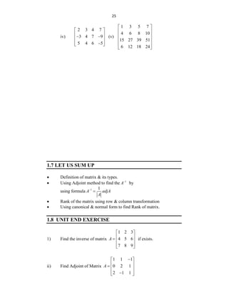
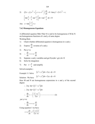
(iii) Adding non-zero scalar multitudes of all the elements of any row
(or columns) into the corresponding elements of any another row (or
column).
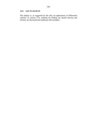
Definition:- Equivalent Matrix:
Two matrices A & B are said to be equivalent if one can be
obtained from the other by a sequence of elementary transformations. Two
equivalent matrices have the same order & the same rank. It can be
denoted by
[it can be read as A equivalent to B]
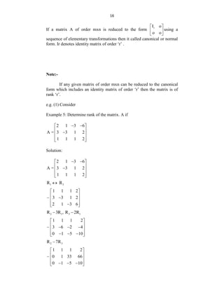
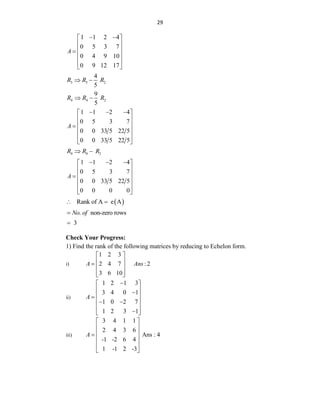
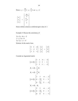
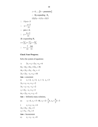
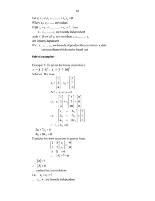
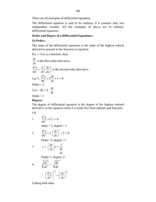
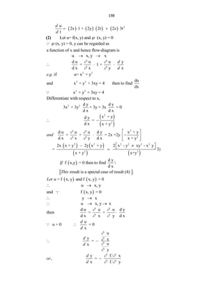
Example 4: Determine the rank of the matrix.
1 2 3
A = 1 4 2
2 6 5
 
 
 
 
 
Solution:
Given
1 2 3
= 1 4 2
2 6 5
A
 
 
 
 
 
2 2 1 3 3 1
R R - R & R R -2R
 
1 2 3
0 2 1
0 2 1
 
 

 
 

 
Here two column are Identical . hence 3rd
order minor of A vanished
Hence 2nd
order minor
1 3
1 0
0 1
 
  
 

 
e(A) 2
 
Hence the rank of the given matrix is 2.
1.5 CANONICAL FORM OR NORMAL FORM

16. 16
If a matrix A of order mxn is reduced to the form r
I o
o o
 
 
 
using a
sequence of elementary transformations then it called canonical or normal
form. Ir denotes identity matrix of order „r‟ .
Note:-
If any given matrix of order mxn can be reduced to the canonical
form which includes an identity matrix of order „r‟ then the matrix is of
rank „r‟.
e.g. (1) Consider
Example 5: Determine rank of the matrix. A if
2 1 3 6
A = 3 3 1 2
1 1 1 2
 
 
 

 
 
 
Solution:
2 1 3 6
A = 3 3 1 2
1 1 1 2
 
 
 

 
 
 
1 3
R R

1 1 1 2
3 3 1 2
2 1 3 6
 
 

 
 

 
2 1 3 1
R 3R , R 2R
 
1 1 1 2
3 6 2 4
0 1 5 10
 
 
  
 
 
  
 
2 3
R 7R

1 1 1 2
0 1 33 66
0 1 5 10
 
 
 
 
  
 

17. 17
1 2 3 2
R R , R R
 
1 0 32 64
0 1 33 66
0 0 28 56
 
 
 
 
 

 
3
1
R
28

1 0 32 64
0 1 33 66
0 0 1 2
 
 
 
 
 

 
1 3 2 3
R 32 R , R 33 R
 
1 0 0 0
0 1 0 0
0 0 1 0
 
 
 
 
 
 
3
I o
 Rank of A=3
Example 6: Determine the rank of matrix
1 2 7
A = 2 4 7
3 6 10
 
 
 
 
 
Solution:
1 2 3
A = 2 4 7
3 6 10
 
 
 
 
 
2 1 3 1
R 2R , R 3R
 
1 2 3
2 4 7
3 6 10
 
 
 
 
 
3 2
R R

1 2 3
0 0 1
0 0 0
 
 
 
 
 
1 2
R 3R


18. 18
1 2 0
0 0 1
0 0 0
 
 
 
 
 
2 1
C 2C

1 0 0
0 0 1
0 0 0
 
 
 
 
 
1 3
C C

1 0 0
0 1 0
0 0 0
 
 
 
 
 
 
2
I 0
 Rank of A= 2
Example 7: Determine the rank of matrix A if
1 1 2 4
2 3 1 1
A =
3 1 3 2
6 3 0 7
  
 
 
 
 
 

 

 
Solution:
1 1 2 4
2 3 1 1
A =
3 1 3 2
6 3 0 7
  
 
 
 
 
 

 

 
2 1 3 1 4 1
R 2R , R 3R , R 6R ,
  
1 1 2 4
0 5 3 7
0 4 9 10
0 9 12 17
  
 
 
 
 
 
 
2 3
R R


19. 19
1 1 2 4
0 1 6 3
0 4 9 10
0 9 12 17
  
 
 
 
 
 
 
 
1 2 3 2 4 2
R + R , R 4R , R 9R
 
1 0 8 7
0 1 6 3
0 0 33 22
0 0 66 44
 
 
 
 
 
 
 
 
4 3
R 2R

1 0 8 7
0 1 6 3
0 0 33 22
0 0 0 0
 
 
 
 
 
 
 
 
3
1
R
11

1 0 8 7
0 1 6 2
0 0 3 2
0 0 0 0
 
 
 
 
 
 
 
 
3 4
C - C
1 0 1 7
0 1 3 3
0 0 1 2
0 0 0 0
 
 
 
 
 
 
 
 
1 3 2 3
R + R , R 3R

1 0 0 5
0 1 0 3
0 0 1 2
0 0 0 0

 
 
 
 
 
 
 
4 1 2 2
C - 5C 3C 2C
 
1 0 0 0
0 1 0 0
0 0 1 0
0 0 0 0
 
 
 
 
 
 

20. 20
3
I 0
0 0
 
 
 
 Rank of A= 3
Check Your Progress:-
Reduce the following to normal form and hence find the ranks of the
matrices.
i)
1 2 3
3 1 2
 
 
 
ii)
2 3 4
4 3 1
1 2 4
iii)
3 4 6
5 5 7
3 1 4



iv)
1 2 3 0
2 4 3 2
3 2 1 3
6 8 7 5
v)
2 1 3 6
3 3 1 1
1 1 1 2
 
 vi)
1 2 1 0
3 2 1 2
2 1 2 5
5 6 3 2
1 3 1 3

 
vii)
2 6 2 6 10
3 3 3 3 3
1 2 4 3 5
2 0 4 6 10
1 0 2 3 5

   
 viii)
3 4 5 6 7
4 5 6 7 8
5 6 7 8 9
10 11 12 13 14
15 16 17 18 19
1.6 NORMAL FORM PAQ
If A is any mxn matrix „r‟ then there exist non singular matrices P and Q
such that,
r
I 0
PAQ
0 0
 

 
 
We observe that, the matrix A can be expressed as
A = Im In …………(i)
Where Im In are the identity matrices of order m and n respectively.
Applying the elementary transformations on this equation. A in L.H.S.
can be reduced to normal form. The equation can be transformal into the
equations.
r
I 0
PAQ
0 0
 

 
 
…………(ii)

21. 21
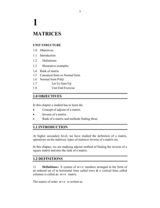
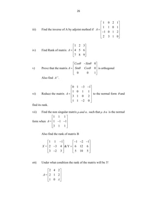
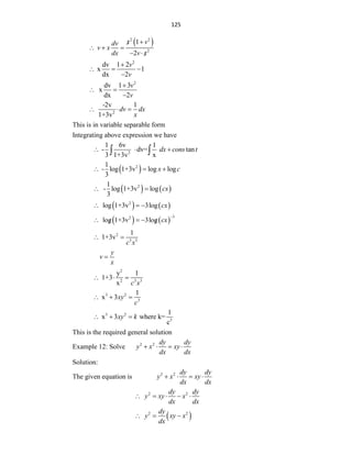
Note that, the row operations can be performed simultaneously on L.H.S.
and prefactor (i.e. Im in equation (i)) and column operations can be
performed simultaneously on L.H.S. and post factor in R.H.S. i.e. [(In in
eqn (i)]
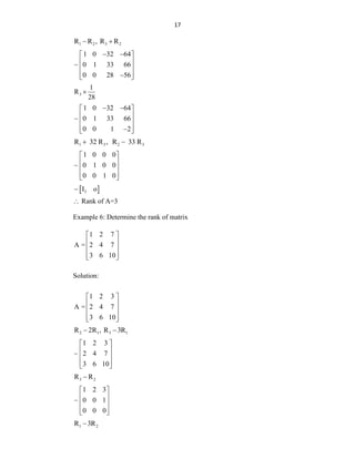
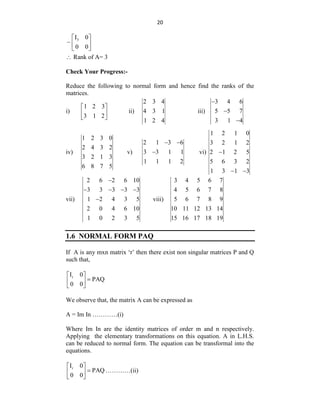
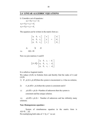
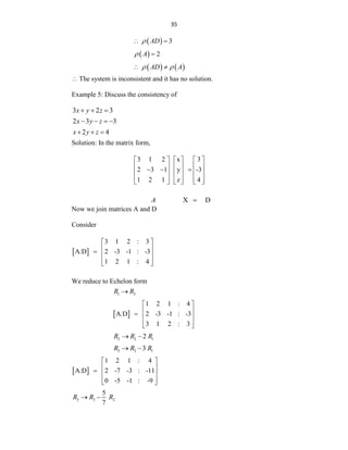
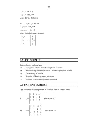
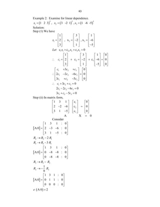
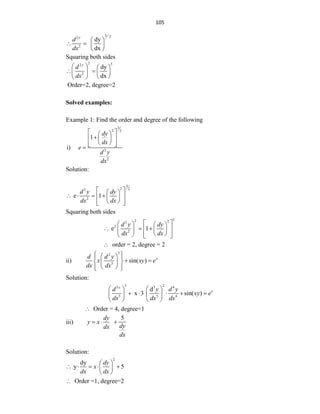
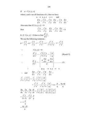
Examples 8: Find the non-singular matrices P and Q such that PAQ is in
normal and hence find the rank of A.
i)
2 1 3
A 3 4 1
1 5 4

 
 
 
 
 

 
Solution: Consider
A= I3 AI 3
2 1 3 1 0 0 1 0 0
3 4 1 = 0 1 0 A 0 1 0
1 5 4 0 0 1 0 0 1

     
     

     
     

     
1 3
R R

1 5 4 0 0 1 1 0 0
3 4 1 = 0 1 0 A 0 1 0
2 1 3 1 0 0 0 0 1

     
     

     
     

     
2 3 1
C 5C , C 4C
 
1 0 0 0 0 1 1 5 4
3 11 11 = 0 1 0 A 0 1 0
2 11 11 1 0 0 0 0 1

     
     
 
     
     
 
     
2 3
R R

1 0 0 0 0 1 1 5 4
1 0 0 = 1 1 0 A 0 1 0
2 11 11 1 0 0 0 0 1

     
     

     
     
 
     
2 1 3 1
R R , R 2R ,
 
1 0 0 0 0 1 1 5 4
0 0 0 = 1 1 1 A 0 1 0
0 11 11 1 0 2 0 0 1

     
     
 
     
     
 
     
3 2
C C


22. 22
1 0 0 0 0 1 1 5 1
0 0 0 = 1 1 1 A 0 1 1
0 11 0 1 0 2 0 0 1
 
     
     
 
     
     
 
     
3
1
R ,
11

1 0 0 0 0 1 1 5 1
0 0 0 = 1 1 1 A 0 1 1
0 1 0 1 2 0 0 1
0
11 11
   
   
 
   
 
 
   
 
   

   
 
 
2 3
R R

0 0 1
1 0 0 1 5 1
1 2
0 1 0 = 0 A 0 1 1
11 11
0 0 0 0 0 1
1 1 1
   
   
 
   

 
   
 
   
   
 
 
Thus
0 0 1
1
1 2
P = 0 P =
11 11 11
1 1 1
 
  
 
 
 
 
 
1 5 1
Q = 0 1 1 Q = 1
0 0 1
 
 
  
 
 
 
P and Q are non-singular matrices
Also Rank of A = 2
ii)
2 1 3 6
A 3 3 1 2
1 1 1 2
 
 
 
 
 
 
 
Solutions:
Consider
1 0 0 0
1 0 0
0 1 0 0
A= 0 1 0 A
0 0 1 0
0 0 1
0 0 0 1
 
   
   
   
   
 
 

23. 23
1 0 0 0
2 1 3 6 1 0 0
0 1 0 0
3 3 1 2 0 1 0 A
0 0 1 0
1 1 1 2 0 0 1
0 0 0 1
 
 
     
     
 
     
     
   
 
1 3
R R

1 0 0 0
1 1 1 2 0 0 1
0 1 0 0
3 6 2 4 0 1 0 A
0 0 1 0
2 1 5 10 1 0 0
0 0 0 1
 
     
     
   
     
   
    
   
 
2 1 3 1 4 1
C C , C C , C 2C
  
1 1 1 2
1 0 0 0 0 0 1
0 1 0 0
3 6 2 4 0 1 0 A
0 0 1 0
2 1 5 10 1 0 0
0 0 0 1
  
 
     
     
   
     
   
    
   
 
2 1 3 1
R 3R , R 2R
 
1 1 1 2
1 0 0 0 0 0 1
0 1 0 0
0 6 2 4 0 1 3 A
0 0 1 0
0 1 5 10 1 0 2
0 0 0 1
  
 
     
     
    
     
   
     
   
 
2 3
R 6R ,

1 1 1 2
1 0 0 0 0 0 1
0 1 0 0
0 0 28 56 6 1 9 A
0 0 1 0
0 1 5 10 1 0 2
0 0 0 1
  
 
     
     

     
   
     
   
 
4 3
C 2C

1 1 1 0
1 0 0 0 0 0 1
0 1 0 0
0 0 28 0 6 1 9 A
0 0 1 2
0 1 5 0 1 0 2
0 0 0 1
 
 
     
     
 
     

   
    
   
 
3 2
C 5C

1 1 4 0
1 0 0 0 0 0 1
0 1 5 0
0 0 28 0 6 1 9 A
0 0 1 2
0 1 0 0 1 0 2
0 0 0 1

 
     

     
 
     

   
   
   
 
 
2 3
1
R , R 1
28
  

24. 24
1 1 4 0
0 0 1
1 0 0 0
0 1 5 0
3 9
1
0 0 1 0 A
14 28 28 0 0 1 2
0 1 0 0 1 0 2 0 0 0 1

 
 
   
  
   
  
   

 
   
   
   
2 3
R R

1 1 4 0
1 0 0 0 0 0 1
0 1 5 0
0 1 0 0 1 0 2 A
0 0 1 2
0 0 1 0 3 9
1
0 0 0 1
14 28 28

 
 
   
  
   
 
 
   

 
   
   
   
 
3
1 1 4 0
0 0 1
0 1 5 0
I 0 = 1 0 2 A
0 0 1 2
3 9
1
0 0 0 1
14 28 28

 
 
 
  
 
 
 

 
 
 
   
0 0 1
1
P = 1 0 2 , P
28
3 9
1
14 28 28
 
 
 
 
 
 
 
1 1 4 0
0 1 5 0
Q = , Q 1
0 0 1 2
0 0 0 1

 
 

  
 

 
 
 P&Q are non singular.
Also,
Rank of A = 3.
Check Your Progress:
A) Find the non-singular matrices P and Q such that PAQ is in normal
form and hence find rank of matrix A.
i)
1 0 2
2 3 4
3 3 6

 
 

 
 

 
ii)
1 2 3 2
2 3 5 1
1 3 4 5
 
 
 
 
 
iii)
3 1 1
1 1 1
1 1 1
 
 
 
 

 

25. 25
iv)
2 3 4 7
3 4 7 9
5 4 6 5
 
 
 
 
 

 
(v)
1 3 5 7
4 6 8 10
15 27 39 51
6 12 18 24
 
 
 
 
 
 
1.7 LET US SUM UP
 Definition of matrix & its types.
 Using Adjoint method to find the 1
A
by
using formula 1 1
A adjA
A


 Rank of the matrix using row & column transformation
 Using canonical & normal form to find Rank of matrix.
1.8 UNIT END EXERCISE
1) Find the inverse of matrix
1 2 3
4 5 6
7 8 9
A
 
 
  
 
 
if exists.
ii) Find Adjoint of Matrix
1 1 1
0 2 1
2 1 1
A

 
 
  
 

 

26. 26
iii) Find the inverse of A by adjoint method if
1 0 2 1
1 1 0 1
1 0 1 2
2 3 1 0
A
 
 
 

 

 
 
iv) Find Rank of matrix
1 2 3
4 5 6
7 8 9
A
 
 
  
 
 
v) Prove that the matrix
0
0
0 0 1
Cos Sin
A Sin Cos

 
 
  
 
 
 
  is orthogonal
Also find 1
.
A
vi) Reduce the matrix
0 1 3 1
1 0 1 1
3 1 0 2
1 1 2 0
A
 
 
 
 

 
 

 
to the normal form  and
find its rank.
vii) Find the non singular matrix ρ and α . such that ρ Aα is the normal
form when
1 1 1
1 1 1
3 1 1
A=
 
 
 
 
 
 
Also find the rank of matrix B
1 1 1 1 2 1
2 3 4 &Y 6 12 6
3 2 3 5 10 5
X =
   
   
   
 
   
   

   
viii) Under what condition the rank of the matrix will be 3!
2 4 2
2 1 2
1 0
A=

 
 
 
 
 

27. 27
ix) If
1 1 1 1 2 1
2 3 4 &Y 6 12 6
3 2 3 5 10 5
X =
   
   
   
 
   
   

   
Then show that    
xy yx
 
 where  denotes Rank.
x) Find the rank of matrix
8 3 6 1
1 6 4 2
7 9 10 3
15 12 16 4
A=
 
 

 
 
 
 
*****
2
LINEAR ALGEBRIC EQUATIONS
UNIT STRUCTURE
2.1 Objectives
2.2 Introduction
2.3 Canonical or echelon form of matrix
2.4 Linear Algebraic Equations
2.5 Let Us Sum Up
2.6 Unit End Exercise
2.1 OBJECTIVES
After going through this chapter you will be able to
- Find the rank of Matrix.
- Find solution for linear equations.
- Type of linear equations.
- Find solution for Homogeneous equations.
- Find solution of non-Homogeneous equations.
2.2 INTRODUCTION
In XIIth we have solved linear equations by using method of
reduction also by rule. Here we are going to find solution of homogeneous

28. 28
and non-homogeneous both with different case. Using matrix we can
discuss consistency of system of equation.
2.3 CACONICAL OR ECHOLON FORM OF MATRIX
Let A be a given matrix. Then the canonical or Echelon form of A is a
matrix in which
(i) One or more elements in each of first r-rows are non-zero and
these first r-rows form an upper triangular matrix.
(ii) The elements in the remaining rows are zero.
Note :
1) The number of non-zero rows in Echelon form is the rank of the
matrix.
2) To reduce the matrix to Echelon form only row transformations are
to be applied.
Solved Examples :-
Example 1: Reduce the matrix to Echelon and find its rank.
2 3 -1 1
1 -1 -2 4
3 1 3 2
6 3 0 7
A

 
 
 
 

 

 

 
Solution:
2 3 -1 1
1 -1 -2 4
3 1 3 2
6 3 0 7
A

 
 
 
 

 

 

 
1 2
R R

1 -1 -2 4
2 3 -1 1
3 1 3 2
6 3 0 7
A

 
 

 

 

 

 
2 2 1
2
R R R
 
3 3 1
3
R R R
 
4 4 1
6
R R R
 

29. 29
1 1 2 4
0 5 3 7
0 4 9 10
0 9 12 17
A
 
 
 
 

 
 
 
3 3 2
4
5
R R R
 
4 4 2
9
5
R R R
 
1 1 2 4
0 5 3 7
0 0 33 5 22 5
0 0 33 5 22 5
A
  
 
 
 

 
 
 
4 4 3
R R R
 
1 1 2 4
0 5 3 7
0 0 33 5 22 5
0 0 0 0
A
  
 
 
 

 
 
 
 
Rank of A e A
 
. non-zero rows
No of

3

Check Your Progress:
1) Find the rank of the following matrices by reducing to Echelon form.
i)
1 2 3
2 4 7 : 2
3 6 10
A Ans
 
 
  
 
 
ii)
1 2 1 3
3 4 0 1
1 0 2 7
1 2 3 1
A

 
 

 

 
 
 

 
iii)
3 4 1 1
2 4 3 6
Ans : 4
-1 -2 6 4
1 -1 2 -3
A
 
 
 

 
 
 

30. 30
2.4 LINEAR ALGEBRIC EQUATIONS
i) Consider a set of equations :
1 1 1 1
a x b y c z d
  
2 2 2 2
a x b y c z d
  
3 3 3 3
a x b y c z d
  
The equation can be written in the matrix form as :
1 1 1 1
2 2 2 2
3 3 3 3
x
y
a b c d
a b c d
a b c z d
     
     

     
     
     
A X D
. . AX D
i e 
Now we join matrices A and D
 
1 1 1 1
2 2 2 2
3 3 3 3
:
: :
:
a b c d
A D a b c d
a b c d
 
 
  
 
 
It is called as Augment matrix
We reduce (A.D.) to Echelon form and thereby find the ranks of A and
(A:D)
1) If ( ) ( )
A AD
 
 then the system is inconsistent i.e. it has no solution.
2) If ( ) ( )
AD A
 
 then the system is consistent and if
(i) ( ) ( )
AD A
 
 Number of unknowns then the system is
consistent and has unique solution.
(ii) ( ) ( )
AD A
 
  Number of unknowns and has infinitely many
solutions.
Non- Homogeneous equation:-
System of simultaneous equation in the matrix form is
AX=D…..(I)
Pre-multiplying both sides of I by 1
A
we set

31. 31
1 1
A AX A D
 
 
1
IX A B

 
1
X A B

 
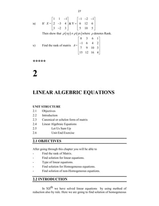
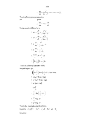
which is required solution of the given non-homogeneous equation.
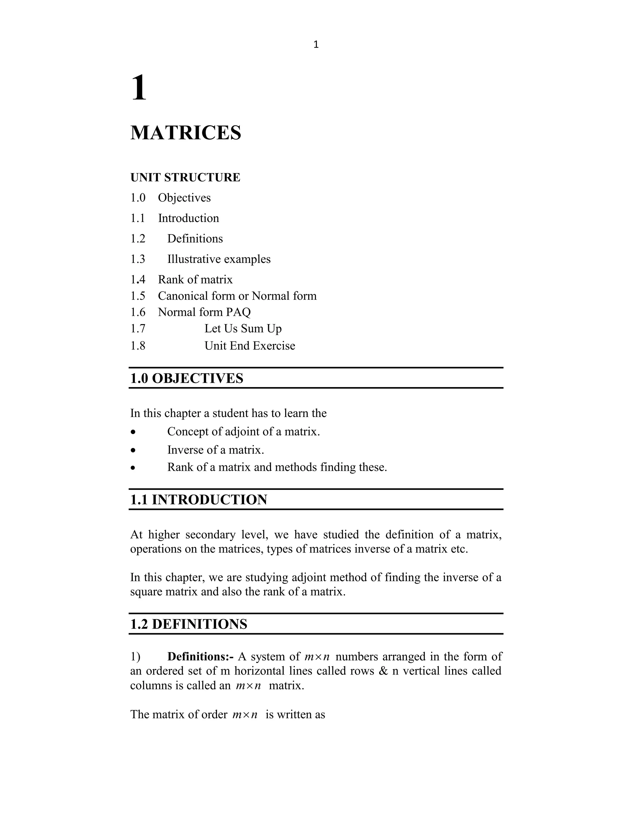
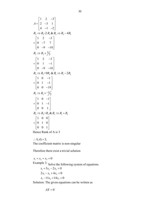
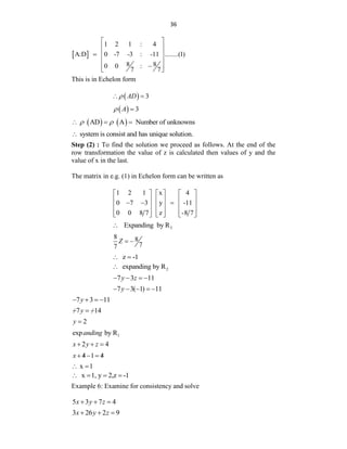
Homogeneous linear equation:-
Consider the system of simultaneous equations in the matrix form.
AX D

If all elements of D are zero
i.e
then the system of equation is known as homogeneous system of
equations.
In this case coefficient matrix A and the augmented matrix [A,O]
are the same. So The rank is same. It follow that the system has solution
1 2 3 4
, , ....... 0,
x x x x  which is called a trivial solution.
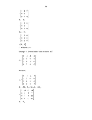
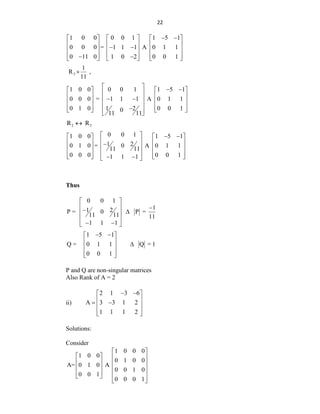
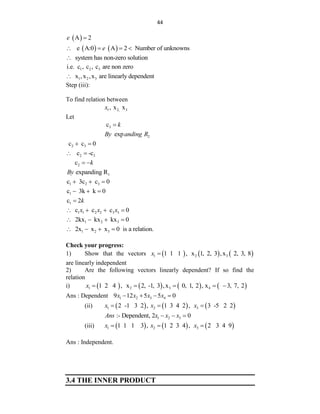
Example 2: Solve the following system of equations
1 2 3
2 3 0
x x x
  
1 2 3
2 3 0
x x x
  
1 2 3
4 2 0
x x x
  
Solution: The system is written as
0
AX 
1
2
3
2 3 1 x 0
1 2 3 0
4 1 2 0
x
x
     
     
 
     
     
 
     
Hence the coefficient and augmented matrix are the same
We consider
2 3 1
1 2 3
4 1 2
A

 
 
 
 
 
 
 
2 3 1
1 2 3
4 1 2
A

 
 
 
 
 
 
 
1 1 2
R R R
 

32. 32
1 2 3
2 3 1
4 1 2
A

 
 
 
 
 
 
 
2 2 1 3 3 1
-2 & 4
R R R R R R
  
1 2 3
0 7 7
0 9 10

 
 
 
 
 
 
 
2 2
1
7
R R
 
1 2 3
0 1 1
0 9 10

 
 
 
 
 
 
 
3 3 2 1 1 2
+9 & 2
R R R R R R
  
1 0 1
0 1 1
0 0 19

 
 
 
 
 

 
3 3
1
7
R R 
 
1 0 1
0 1 1
0 0 1

 
 
 
 
 
 
2 2 3 1 1 3
+ &
R R R R R R
  
1 0 0
0 1 0
0 0 1
 
 
  
 
 
Hence Rank of A is 3
( ) 3,
A
 
The coefficient matrix is non-singular
Therefore there exist a trivial solution
1 2 3 0
x x x
  
Example 3:
Solve the following system of equations
1 2 3
3 2 0
x x x
  
1 2 3
2 4 0
x x x
  
1 2 3
11 14 0
x x x
  
Solution: The given equations can be written as
0
AX 

33. 33
1
2
3
1 3 2 x 0
2 1 4 0
1 11 14 0
x
x

     
     
 
     
     
     
Here the coefficient & augmented matrix are the same
1 3 2
2 1 4
1 11 14
A

 
 
 
 
 

 
2 2 1 3 3 1
-2 &
R R R R R R
  
1 3 2
0 7 8
0 14 16

 
 

 
 

 
3 3 2
2
R R R
 
1 3 2
0 7 8
0 0 0

 
 

 
 
 
Here rank of A is 2 i.e
( ) 2
A 
So the system has infinite non-trivial solutions.
1
2
3
1 3 2 x 0
0 7 8 0
0 0 0 0
x
x

     
     
  
     
     
     
1 2 3
3 2 0
x x x
  
2 3
7 8 0
x x
  
2 3
7 8
x x

2 3
8
7
x x

Let 3 3
8
x x 
 
2
8
7
x 
 
1
8
3 2 0
7
x  
 
   
 
 
1
24
2 0
7
x  
   
1
24
2
7
x  
  
1
10
7
x 
  

34. 34
Hence 1
10
7
x 
  2
8
7
x 
 and 3
x 

1
2
3
10
7
x
8
7
x
x



 

 
   
   

   
   
 
 
 
 
Hence infinite solution as deferred upon value of 
Example 4: Discuss the consistency of
2 3 4 2
x y z
   
3 4
x y z
  
3 2 5
x y z
   
Solution: In the matrix form
2 3 4 x -2
1 1 3 y 4
3 2 1 z -5

     
     
 
     
     

     
Consider an Agumental matrix
 
2 3 4 : 2
: 1 1 3 : 4
3 2 1 : 5
A D
 
 
 
 
 
 
 
 
2 2 1
1
2
R R R
 
3 3 1
3
2
R R R
 
 
2 3 4 : 2
5
: 0 5 : 5
2
5
0 5 : 2
2
A D
 
 
 
 
 
 
 
 
 
2 3 2
R R R
 
 
2 3 4 : 2
5
: 0 5 : 5
2
0 0 5 : 7
A D
 
 
 
 
 
 

 

35. 35
   3
AD
 
  2
A
 
    
AD A
 

 The system is inconsistent and it has no solution.
Example 5: Discuss the consistency of
3 2 3
x y z
  
2 3 3
x y z
   
2 4
x y z
  
Solution: In the matrix form,
3 1 2 x 3
2 3 1 y -3
1 2 1 z 4
     
     
  
     
     
     
X D
A 
Now we join matrices A and D
Consider
 
3 1 2 : 3
A:D 2 -3 -1 : -3
1 2 1 : 4
 
 
  
 
 
We reduce to Echelon form
1 3
R R

 
1 2 1 : 4
A:D 2 -3 -1 : -3
3 1 2 : 3
 
 
  
 
 
2 2 1
2
R R R
 
3 3 1
3
R R R
 
 
1 2 1 : 4
A:D 2 -7 -3 : -11
0 -5 -1 : -9
 
 
  
 
 
3 3 2
5
7
R R R
 

36. 36
 
1 2 1 : 4
A:D 0 -7 -3 : -11 ........(1)
8 8
0 0 :
7 7
 
 
 

 

 
 
This is in Echelon form
  3
AD

 
  3
A
 
   
AD A Number of unknowns
 
  
system is consist and has unique solution.

Step (2) : To find the solution we proceed as follows. At the end of the
row transformation the value of z is calculated then values of y and the
value of x in the last.
The matrix in e.g. (1) in Echelon form can be written as
1 2 1 x 4
0 7 3 y -11
0 0 8 7 z -8 7
     
     
  
     
     
     
3
Expanding by R

8 8
7
7
Z  
z -1
 
2
expanding by R

7 3 11
y z
   
7 3( 1) 11
y
    
7 3 11
y
   
7 14
y
  
 
2
y 
1
exp by R
anding
2 4
x y z
  
4 1 4
x  
  
x 1
 
x 1, y 2,z -1
   
Example 6: Examine for consistency and solve
5 3 7 4
x y z
  
3 26 2 9
x y z
  

37. 37
7 2 10 5
x y z
  
Solution:
Step (1) : In the matrix form
5 3 7 x 4
3 26 2 y 5
7 2 10 z 6
     
     

     
     
     
X D
A 
Consider
 
5 3 7 : 4 x 4
: 3 26 2 : 9 y 5
7 2 10 : 5 z 6
A D
     
     
 
     
     
     
1 1
1
R
5
R

 
1 3 5 7 5 : 4 5
: 3 26 2 : 9
7 2 10 : 5
A D
 
 
  
 
 
2 2 1
R 3
R R
 
3 3 1
R 7 R
R
 
 
1 3 5 7 5 : 4 5
: 0 121 5 11 5 : 33 5
0 11 5 1 5 : 3 5
A D
 
 
 
 
 
 
 
3 3 2
1
R R
11
R
 
 
3 7 4
1 :
5 5 5
33
121 11
: 0 :
5 5 5
0 0 0 : 0
A D
 
 
 


 
 
 
 
 
AD 2

 
 
A 2
 
   
AD 2 3 of unknowns
A Number
 
    
The system is consistent and has infinitely many solutions.
Step (2) :- To find the solution we proceed as follows:
Let

38. 38
 
....... parameter
z k k
 
2
By expanding R

121 5 11 5 33 5
y z
 
11y-z 3
 
z 3
y
11

 
put z k
 
k 3
y
11

 
1
R
By exapanding
3 7 4
5 5 5
x y z
  
7 16
x
11 11
k
  
Check Your Progress:
Solve the system of equations:
i) 1 2 3 4
2 2 6
x x x x
   
1 2 3 4
6 6 6 12 36
x x x x
   
1 2 3 4
4 3 3 3 1
x x x x
    
1 2 3 4
2 2 10
x x x x
   
Ans : consistent
ii) 1 2 3 4
2, 1, 1, 3
x x x x
    
1 2 3 4
2 2
x x x x
   
1 2 3 4
3 2
x x x x
   
1 2 3 4
2 1
x x x x
   
1 2 3 4
6 2 5
x x x x
   
Ans : Infinitely many solutions,
iii) 1 2 3 4
5 9
, 3 4 , 2 , 3
2 2
x k x k x k x k
      
3 1 2 3 4
x x x
  
1 2 3
2 5 2 3
x x x
  
1 2 3
7 7 5
x x x
  
Ans : Inconsistent
iv) 1 2 3 0
x x x
  

39. 39
1 2 3
2 0
x x x
  
1 2 3
2 3 0
x x x
  
Ans: Trivial Solution.
v) 1 2 3
2 3 0
x x x
  
1 2 3
2 4 7 0
x x x
  
1 2 3
3 6 10 0
x x x
  
Ans : Definitely many solution
1
2
3
x
1
2
0
x
x


 
   

   

   
 
   
 
2.5 LET US SUM UP
In this chapter we have learn
 Using row echelon from finding Rank of matrix.
 Representing linear equation m x n in to argumented matrix.
 Consistency of matrix.
 Solution of Homogeneous equations.
 Solution of non homogeneous equations.
2.6 UNIT END EXERCISE
1) Reduce the following matrix in Echolon form & find its Rank.
i)
1 3 6 1
1 4 5 1
1 5 4 3
A Ans : Rank = 2

 
 
 

 
 
 
ii)
1 2 1 3
4 1 2 1
3 1 1 2
1 2 0 1
A Ans : Rank = 3

 
 
 

 

 
 

40. 40
iii)
1 2 3
2 1 0
0 1 2
A Ans : Rank = 2
 
 
  
 
 
iv)
1 1 1
1 1 1
3 1 1
A Ans : Rank = 2
 
 
  
 
 
 
2) Solve the following system of equations.
i) 1 2 3 2 3 1 2 3
x +x +x = 3, x+2x +3x = 4, x +4x +9x =6
Ans:- 2, 1, 0.
x y z
  
ii) 1 2 3 1 3 1 2 3
2x - x - x =0, x - x =0, 2x +x -3x =0
Ans:- 1 2 3
1
..... 1 .
1
x x x  
 
 
     
 
  .
iii) 1 2 3 4
5x -3x -7x +x =10
1 2 3 4
-x +2x +6x -3x = -3
1 2 3 4
x +x +4x -5x =0
iii) 1 2 3
2x +3x - 2x =0
1 2 3
3x - x +3x =0
1 2 3
7x +5x - x =0.
iv) 1 2 3
x -4x - x = 3
1 2 3
3x +x -2x =7
1 2 3
2x -3x +x =10.
v) 1 2 3
x -4x +7x = 8
1 2 3
3x +8x -2x =6
1 2 3
7x -8x +26x = 31
*****

41. 41
3
LINEAR DEPENDANCE AND
INDEPENDANCE
OF VECTORS
UNIT STRUCTURE
3.1 Objectives
3.2 Introduction
3.3 Definitions
3.4 The Inner Product
3.5 Eigen Values and Eigen Vectors
3.6 Summary
3.7 Unit End Exercise
3.1 Objectives
After going through this chapter you will able to
 Find linearly independent & linearly dependent vector.
 Inner product of two vector
 Find characteristic equation of matrix
 Find the of characteristic equation i.e
 Find the corresponding .Eigen vector to Eigen value.
3.2 Introduction
In this chapter we are going to discuss linearly dependent &
independent also. Inner two vector using the characteristic equation of
matrix. We are going to evaluate .Eigen value & Eigen.vector of matrix A.
Vector :- An set of n elements written as  
1 2 3 4
, , , ,............. n
x x x x x x

is
called a vector of n-dimensions.
Note : Any two or column matrix is called as a vector and numbers are
called as scalars.
3.3 Definitions
Linearly Independent Vector
Let
1 2
, ,............. be n vectors of some order
n
Let x x x

42. 42
1 1 2 2 n
Let c c ........... c 0
n
x x x
   
1 2
c , , ...... are scalars.
Where c
1 2 n
If (i) c .............. c 0 then
c
   
1 2
x , , ........ are linearly independent
n
x x
i 1 2
and (ii) if not all c are zero then , ,.......... n
x x x
are linearly dependent
1 2
If x , ,......... are linearly dependent then a relation exists
n
x x
between them which can be found out
Solved examples:-
Example 1: Examine for linear dependence
   
1 2
1 2 4 , x 3 7 10
T T
x  
Solution: We have,
1 2
1 3
2 , x 7
4 10
x
   
   
 
   
   
   
1 1 2 0
Let c x c x
 
1 2
1 3 0
. . 2 7 0
4 10 0
i e c c
     
     
 
     
     
     
1 1
1 2
1 2
3 0
. . 2 7 0
4 10 0
c c
i e c c
c c

   
   
 
   
   

   
1 2
3 0
c c
  
1 2
2 7 0
c c
 
1 2
4 10 0
c c
 
Consider first two equations in matrix form.
1
2
1 3 0
2 7 0
c
c
 
   

 
   
   
 
X 0
A 
A 7 6
  
A 1

A 0
 
system has zero solution.

1 2
i.e. c 0
c
 
1 2
x , x are linearly independent


43. 43
Example 2: Examine for linear dependence.
     
1 2 3
1 2 3 , 3 -2 1 , 1 -6 -5
T T T
x x x
  
Solution:
Step (1) We have
1 2 3
1 3 1
2 , x 2 , x 6
3 1 5
x
     
     
    
     
     

     
1 1 21 2 3 3
c c c 0
Let x x x
  
1 2 3
1 3 1 0
2 c 2 c 6 0
3 1 5 0
c
       
       
       
       
       

       
1 2 3
1 2 3
1 2 3
3 0
2 2 6 0
3 5 0
c c c
c c c
c c c
 
   
   
   
   
   
 
   
1 2 3
3 0
c c c
   
1 2 3
2 2 6 0
c c c
  
1 2 3
3 5 0
c c c
  
Step (ii) In matrix form,
1
2
3
1 3 1 c 0
2 2 6 c 0
3 1 5 c 0
     
     
  
     
     

     
A X 0

Consider
 
1 3 1 : 0
A:0 2 3 6 : 0
3 1 5 : 0
 
 
  
 
 

 
2 2 1
2
R R R
 
3 3 1
3
R R R
 
 
1 3 1 : 0
A:0 0 8 8 : 0
0 8 8 : 0
 
 
  
 
 
 
 
3 3 2
R R R
 
2 2
1
8
R R
 
 
1 3 1 : 0
A:0 0 1 1 : 0
0 0 0 : 0
 
 
  
 
 
 
A 0 2
e 

44. 44
 
A 2
e 
   
e A:0 A 2 Number of unknowns
e
   
system has non-zero solution

1 2 3
i.e. c , c , c are non zero
1 2 3
x ,x ,x are linearly dependent

Step (iii):
To find relation between
1 2, 3
, x x
x
Let
3
c k

2
exp
By anding R
2 3
c c 0
 
2 3
c -c
 
2
c k
 
1
expanding R
By
1 2 3
c 3c c 0
  
1
c 3k k 0
  
1
c 2k

1 1 2 2 3 3
c c c 0
x x x
   
1 2 3
2kx kx kx 0
   
1 2 3
2x x x 0 is a relation.
   
Check your progress:
1) Show that the vectors      
1 2 3
1 1 1 , x 1, 2, 3 ,x 2, 3, 8
x 
are linearly independent
2) Are the following vectors linearly dependent? If so find the
relation
i)        
1 2 3 4
1 2 4 , x 2, -1, 3 ,x 0, 1, 2 , x 3, 7, 2
x     
Ans : Dependent 1 2 3 4
9 12 5 5 0
x x x x
   
(ii)      
1 2 3
2 -1 3 2 , 1 3 4 2 , 3 -5 2 2
x x x
  
1 2 3
:- Dependent, 2 0
Ans x x x
  
(iii)      
1 2 3
1 1 1 3 , 1 2 3 4 , 2 3 4 9
x x x
  
Ans : Independent.
3.4 THE INNER PRODUCT

45. 45
If 1 2
( , ....... )
n
X x x x
 and 1 2
( , ....... )
n
Y y y y

then<X,Y> denotes inner product
1 1 2 2 3 3
, ........ n n
X Y x y x y x y x y
      is in inner product of X and Y.
Let V be a vector space and X,Y V then<X,Y> it said to be an inner
product if it satisfies following properties.
i) <X,Y> =0
ii) <X,Y> = <Y,X>
iii) <X,Y+Z> = <X,Y> + <X,Z>
iv) <X, Y> =  <X,Y> where  is scalar.
v) <X,Y> = 0 if and only if X=0.
Example 3: Show that 1 1 2 2 3 3
, 2 4
X Y x y x y x y
   
Satisfies all properties of inner product
Solution: 1 1 2 2 3 3
, 2 4
X Y x y x y x y
   
i) 1 1 2 2 3 3
, 2 4
X Y x y x y x y
   
2 2 2
1 2 3
( ) 2( ) 4( ) 0
x x x
   
, 0
X Y
 
2 2 2
1 2 3
, 0( ) 2( ) 4( ) 0
X Y x x x
    
1 2 3
0, 0, 0
x x orx
  
, 0 0
X X x
  
ii) 1 1 2 2 3 3
, 2 4
X Y x y x y x y
   
1 1 2 2 3 3
2 4
y x y x y x
  
,
Y X
 
iii) 1 1 1 2 2 2 3 3 3
, ( ) 2 ( ) 4 ( )
X Y Z x y z x y z x y z
       
1 1 1 1 2 2 2 2 3 3 3 3
2 2 4 4
x y x z x y x z x y x z
     
1 1 2 2 3 3 1 1 2 2 3 3
2 4 2 4
x y x y x y x z x z x z
     
, ,
X Y X Z
    
iv) 1 1 2 2 3 3
, ( ) 2 ( ) 4 ( )
X Y x y x y x y
   
    
1 1 2 2 3 3
2 4
x y x y x y
  
  
1 1 2 2 3 3
( 2 4 )
x y x y x y

  
,
x y

  
Here all properties are satisfied
,
X Y
  is an inner product.
Check Your Progress:
Prove all the properties of an inner product for the following:-
i. 1 1 2 2
, 16 25
X Y x y x y
  
ii. 1 1 2 2 3 3
, 8
X Y x y x y x y
   

46. 46
iii. 1 1 2 2 3 3
, 3 4
X Y x y x y x y
   
iv. , ( ). ( ).
b
a
f g f t g t dt

 
3.5 Eigen Values And Eigen Vectors
Definition:-
Let A be a given square matrix.
Then there exists a scalar  and non-zero vector X such that
..........(1)
AX X


Our aim is to find and x for given matrix A using equation (1)
 is called as eigen value, latent roots of a matrix value, characteristic
value or root of a matrix A and x is called as eigen vector or characteristic
vector etc.
X is a column matrix
Method of finding  and x :-
We have,
AX X


 
AX- IX 0..... x IX, I unit matrix

   
 
A- I 0.............(2)
X

 
Equation 2 is a set of homogenous equation and for non-zero x, we have
0..........(3)
A I

 
This equation is called the characteristic equation of
First we solve equation (3) to find eigen values or roots. Then we solve
equation (2) to find Eigen vectors.
Let
1 1 1 1
2 2 2 2
3 3 3 3
and x
a b c x
A a b c x
a b c x
   
   
 
   
   
   
 
(2) i.e. A- I 0 becomes
equation x
 
1 1 1 1
2 2 2 2
3 3 3 3
1 0 0 0
0 1 0 0
0 0 1 0
a b c x
a b c x
a b c x

 
       
 
       
 
 
       
 
       
       
 

47. 47
1 1 1 1
2 2 2 2
3 3 3 3
0
. . 0 (2)
0
a b c x
i e a b c x
a b c x




     
     
  
     
     

     
equation (3) i.e. A- x 0 is
and  
1 1 1
2 2 2
3 3 3
0 (3)
a b c
a b c
a b c




 
 
  
 
 

 
Note :
1) Equation (2) is called as matrix equation of A in 
2) Equation (3) is called as characteristic equation of A in 
3) Usually given matrix A is of order 3X3 . Therefore it will have 3
eigen values and for every eigen value there will be corresponding eigen
vector which is a column matrix of order 3X1. There are 3 such column
matrices.
4) Eigen vectors are linearly independent.
5) Method of finding eigen values is same for any given matrix A.
Method of finding eigen vectors is slightly different and we study 3 types
of such problems.
Type (I) : When all eigen values are distinct and matrix A may be
symmetric or non- symmetric.
Type (II) : When eigen values are repeated and A is non-symmetric
Type (III) : When eigen values are repeated and A is symmetric.
Solved examples :-
Type (I) : All roots are non- repeated.
Example 4: Find eigen values and given vectors for
2 2 3
1 1 1
1 3 1
A

 
 
  
 

 
Solution: (1) : Charactristic equation of A in i s
Step 
A- I 0
 
2- -2 3
. . 1 1- 1 0
1 3 -1-
i e




 
3 2
diagonal elements of A
sum of
 
  
 
minors of diagonal elements of A - A 0
sum of  
     
2 1 3 2 1 1 3 3 1
A
        

48. 48
-8-4 6
 
A 6
 
Characteristic equation is given by
   
3 2
2 4 5 4 - 6 0
  
       
3 2
2 -5 6 0
  
   
sin sum of coefficient 0
ce 
 
-1 is a factor.


Synthetic division:
1 1 -2 -5 6
1 -1 -6
1 -1 -6 0
   
2
-1 6 0
  
   
     
-1 -3 2 0
  
   
1, -2, 3

 
The roots are non- repeated

Step (ii) :- Now we find eigen vectors
Matrix equations is given by
 
I 0
A X

 
1
2
3
2- -2 3 x 0
. . 1 1- 1 x 0
1 3 1 x 0
i e



     
     

     
     
 
     
n
( ): When 1, matrix eq becomes
Case i 
 
1
2
3
1 -2 3 x 0
1 0 1 x 0
1 3 2 x 0
     
     

     
     

     
Solving first two rows by Cramer‟s rule.
We have,
1 2 3
2 3 0
x x x
  
1 2 3 0
x x x
  
3
1 2
x
-2 2 2
x
x

  
 
3
1 2
x
-1 1 1
x
x
  

49. 49
1
1
x 1
1

 
 
   
 
 
Case (ii) :- When 2 2
  
Matrix equation is given by
1
2
3
4 2 3 x 0
1 3 1 x 0
1 3 1 x 0

     
     
     
     
     
3
1 2 x
x x
-11 1 14
  
3
1 2 x
x x
-11 -1 14
  
2
11
x 1
14

 
 
  
 
 
 
Case (iii) : When 3 3
   matrix equation is given by
1
2
3
1 2 3 x 0
1 2 1 x 0
1 3 4 x 0
 
     
     
 
     
     

     
3
1 2 x
x -x
4 4 4
  

3
1 2
3
1
x
x x
x 1
1 1 4
1
 
 
      
 
 
Type (II) :- Repeated eigen values and A is non- symmetric.
Example 5: Find eigen values and eigen vectors for
2 1 1
2 3 2
3 3 4
A
 
 
  
 
 
Solution:
Step (1) :- Characteristic equation of A in  is
 
I 0
A 
 
 
3 2
. . -9 6 5 4 -7 0
i e   
   
3 2
-9 15 -7 0
  
 
since sum of co-efficients 0

 
1 is a factor

 
synthetic division

50. 50
1 1 9 15 7
1 8 7
1 8 7 0
 


2
-8 7
 
 
   
-7 1
 
 
3 2
-9 15 -7 0
  
  
     
-1 1 -7 0
  
  
7, 1, 1
 
Here two roots are repeated. First we find eigen vectors for non-repeated
root.
Step II :- Matrix equation of A in  is
 
I 0
A X

 
1
2
3
2 1 1 x 0
2 3 2 x 0
3 3 4 x 0




     
     
 
     
     

     
Case (i) :- For 7
 
Matrix equation is
1
2
3
5 1 1 x 0
2 4 2 x 0
3 3 3 x 0

     
     
 
     
     

     
3
1 2 x
x -x
6 -12 18
  
3
1 2 x
x x
1 2 3
  
1
1
x 2
3
 
 
   
 
 
Case (ii) :- Let 1
 
Matrix equation is
1
2
3
1 1 1 x 0
2 2 2 x 0
3 3 3 x 0
     
     

     
     
     
By cramers‟s rule we get
3
1 2
0 0 0
x
x x

 
0
. . 0
0
i e
 
 
 
 
 
But by definition we want non-zero x2

51. 51
So we proceed as follows
1
by R
Expanding
1 2 3 0
x x x
  
Assume any element to be zero say x1 and give any conventional value
say 1 to x2 and find x3
Let
1 2
0, x 1
x  
3 1
x
  
2
0
1
1
x
 
 
   
 

 
Case (iii) :- Let x=1
Again consider
1 2 3
x x x 0
  
2 1
0, x 1
Let x  
3 1
x
  
2
0
1
1
x
 
 
   
 

 
Type (iii) :- A is symmetric and eigen values are repeated
Example 6: Find eigen values and eigen vectors for .
6 2 2
2 3 1
2 1 3
A

 
 
  
 
 

 
Solution:
Step :- Characteristic equations of A in  is
  0
A I

 
6 2 2
2 3 1 0
2 1 3



 
 
 
   
 
 
 
 
 
A 32

 
3 2
. . 12 8 14 14 -32 0
i e   
    
3 2
12 36 -32 0
  
   
 
-2 is a factor

Synthetic division :-
2 1 12 36 32
2 20 32
1 10 16 0
 



52. 52
2
10 6
 
 
  
8 2
 
  
3 2
12 36 32 0
  
    
   
2 2 8 0
  
   
8, 2, 2

 
Step (ii) :- Matrix equation is
1
2
3
6 2 2 x 0
2 3 1 x 0
2 1 3 x 0



 
     
     
   
     
     
 
     
Case (i) :- For 8
 
Matrix equation is given by
1
2
3
2 2 2 x 0
2 5 1 x 0
2 1 5 x 0
 
     
     
   
     
     

     
3
1 2
x
........ cramer's rule
12 6 6
x
x
By

  
3
1 2
x
2 1 1
x
x

 

1
2
x 1
1
 
 
  
 
 
 
Case (ii) :- Let 2
 
Matrix equation is given by
1
2
3
4 2 2 0
2 1 1 0
2 1 1 0
x
x
x

     
     
  
     
     

     
1
R
Expanding
1 2 3
4 2 2 0
x x x
  
1 2
x 0, x 1
Let  
3
x 1
 
2
0
x 1
1
 
 
   
 
 
Case (iii) :- Let
2
 
A is symetric

1 2 3
x , x , are orthogonal
x


53. 53
3
Let, x
l
m
n
 
 
  
 
 
1 3
x , x are orthogonal
1
1 3
x , x 0
 
2l-m n 0..........(1)
  
2 3
x , x are orthogonal
1
2 3
x , x 0
 
ol m n 0..........(2)
   
solving (1) and (2) by cramer's rule
l
-2 2 2
m n

 
l
1 1 1
m n
  
 
3
1
x 1
1
 
 
   
 

 
Check your progress:
1) Find eigen values and eigen vectors for
i)
2 8 12
1 4 4
0 0 1
A
  
 
 
  
 
 
Ans :- Eigen values are 0,1,2
2 3
4 4 2
1 x 0 , x 1
0 1 0
x
     
     
     
     
     

     
(ii)
3 1 1
1 5 1
1 1 3
A

 
 
  
 
 

 
Ans are 2,3 and 6
Eigen values
1 2 3
1 1 1
0 x 1 x 2
1 1 1
x

     
     
   
     
     
     

54. 54
(iii)
2 2 3
2 1 6
1 2 0
A
 
 
 
 
 
 

 
Ans : are 5, -3,-3
Eigen values
1 2 3
1 2 3
2 x 1 x 0
1 0 1
x

     
     
  
     
     

     
3.6 SUMMARY
In this chapter we have learn
 Linearly dependent & independent vector.
 Inner product of two vector i.e same as dot product 7 its properties.
 Characteristics equation & its root by using
0
A I

 
 Eigen vector which is corresponding to Eigen value which we get
from 0
A I

 
3.7 UNIT END EXERCISE
1) Is the system of vector 1 2
(2,2,1) , (1,3,1)
T T
x x
  linear
by dependent?
2) Show that the vectors (1,2,3) (2,20) form a linearly
independent set.
3) Show that the following vector are linearly dependent
& find the relation between them
1 2 3
(1, 1,1), (2,1,1), (3,0,2)
x x x
   
4) Prove the properties of an inner product.
i. 1 1 2 2
, 3 4 .
X Y x y x y
  
ii. 1 1 2 2 3 3
, 9 3 4
X Y x y x y x y
   
5) Find Eigen value and Eigen vector for the following
matrix.

55. 55
i)
2 2 0
2 1 1
7 2 3
A
 
 
  
 
 
 
ii)
1 2 4
0 2 4
0 0 3
A
 
 
  
 
 
iii)
1 0
2 4
A
 
  
 
iv)
2 1
8 4
A

 
  

 
v)
1 1 1
1 2 1
3 2 3
A
 
 
  
 
 
vi)
1 3 0
3 2 1
0 1 1
A
 
 
  
 
 

 
vii)
0
0
Cos Sin
A
Sin Cos



 
  
 
viii)
2 2 1
1 3 1
1 2 1
A
 
 
  
 
 
*****

56. 56
4
CAYLEY – HAMILTON THEORY
UNIT STRUCTURE
4.1 Objective
4.2 Introduction
4.3 Cayley – Hamilton Theorem
4.4 Similarity of Matrix
4.5 Characteristics Polynomial
4.6 Minimal Polynomial
4.7 Complex Matrices
4.8 Let Us Sum Up
4.9 Unit End Exercise
4.1 OBJECTIVE
After going through this chapter you will able to
 Find by using Cayley Hamilton Theorem.
 Application of Cayley- Hamilton Theorem.
 Find diagonal matrix on similar matrix.
 Characteristic Polynomial & Minimal Polynomial of matrix A.
 Derogatory & non-derogatory matrix.
 Complex matrix like Hermitian, Skew-Hermitian unitary matrix.
4.2 INTRODUCTION
In previous chapter we learn about Eigen values & Eigen Vector. How
here we are going to discuss Cayley Hamilton Theory & its application
also we had study only Real matrix. We introduce here complex matrix
with type of complex matrix also minimal polynomial.
4.3 CAYLEY – HAMILTON THEOREM
Statement: Every square matrix satisfies its own characteristic equation.
If the characteristic Equation for the nth
order square matrix A is
  1 2
1 2
1 ........
n n n n
n
A I a a a
   
 
 
     
  then
   
1 2
1 2
1 ........ 0
n n n n
n
A a A a A a I
 
    

57. 57
Example 1:
Show that the given matrix A satisfies its characteristic equation.
2 1 1
0 1 0
1 1 2
A
 
 
  
 
 
Solution:
The characteristic equation of the matrix A is 0
A I

 
2 1 1
0 1 0 0
1 1 2




 

        
 
2 1 2 0 1 0 1 0 1 0
   
         
 
 
   
2
2 2 3 1 1 0
   
 
       
 
2 2 3
4 6 2 2 3 1 0
     
        
3 2
5 7 3 0
  
    
3 2
5 7 3 0
  
    
By Cayley Hamilton theorem,
3 2
5 7 3 0
A A A I
    ………………………..(1)
Now, we have
2
2 1 1 2 1 1 5 4 4
0 1 0 0 1 0 0 1 0
1 1 2 1 1 2 4 4 5
A
     
     
 
     
     
     
3
2 1 1 5 4 4 14 13 13
0 1 0 0 1 0 0 1 0
1 1 2 4 4 5 13 13 14
A
     
     
 
     
     
     
3 2
5 7 3
A A A I
    
14 13 13 5 4 4 2 1 1 1 0 0
0 1 0 -5 0 1 0 +7 0 1 0 3 0 1 0
13 13 14 4 4 5 1 1 2 0 0 1
       
       
 
       
       
       

58. 58
14 13 13 5 4 4 2 1 1 1 0 0
0 1 0 -5 0 1 0 +7 0 1 0 3 0 1 0
13 13 14 4 4 5 1 1 2 0 0 1
       
       
 
       
       
       
14 13 13 25 20 20 14 7 7 3 0 0
0 1 0 - 0 5 0 + 0 7 0 0 3 0
13 13 14 20 20 25 7 7 14 0 0 3
       
       
 
       
       
       
28 20 20 28 20 20
0 8 0 0 8 0
20 20 28 20 20 28
   
   
 
   
   
   
0 0 0
0 0 0
0 0 0
 
 
  
 
 
0

3 2
5 7 3 0
A A A I
    
Thus the matrix A satisfies its characteristic equation.
Example 2 :
Calculate 7
A by using Cayley Hamilton theorem.
Where
3 6
A =
1 2
 
 
 
Solution :
The characteristic equation of A is
0
A I

 
3 6
0
1 2



 

 

 
   
3 2 6 0
 
   
2
6 2 3 6 0
    
  
2
5 0
  
 
By Cayley Hamilton theorem,
2
5 0
A A
 
i.e. 2
5
A A


59. 59
Now to calculate
7 5 2 5 6
. .5 5
A A A A A A
  
4 2 5
5 . 25
A A A
 
3 2 4
25 . 125
A A A
 
2 2
125 . 125(5 ).(5 )
A A A A
 
2
3125 3125(5 )
A A
 
15625A

7 3 6
15625
1 2
A
 
  
 
46875 93750
15625 31250
 
  
 
 The value of 7 46875 93750
15625 31250
A
 
  
 
Example 3:
By using Cayley Hamilton theorem find 1
A
1 1 1
1 1 2
1 2 1
A

 
 
 
 
 
 
Solution:
The characteristics equation of A is
0
A I

 
1 1 1
1 1 2 0
1 2 1



 
 
 
  
 
 

 
     
2
1 1 2 4 1 1 2 1 2 1 0
    
 
           
 
2 2 3
2 3 3 2 3 3 0
      
         
3 2
3 3 9 0
  
    
3 2
3 3 9 0
  
   
By Cayley Hamilton theorem
3 2
3 3 9 0
A A A I
   

60. 60
Multiply by 1
A
3 1 2 1 1 1 1
3 3 9 0
A A A A AA IA A
    
    
2 1
3 3 9 0
A A I A
    
1 2
1
3 3
9
A A I A

 
  
  …….(1)
2
1 1 1 1 1 1 3 0 0
1 1 2 1 1 2 0 6 3
1 2 1 1 2 1 0 3 6
A
 
     
     
   
     
     
     
1 1 1 1 0 0 3 0 0
3 3 3 1 1 2 3 0 1 0 0 6 3
1 2 1 0 0 1 0 3 6
A I A

     
     
     
     
     
     
2
3 3 3 3 0 0 3 0 0
3 3 3 3 6 0 3 0 0 6 3
3 6 3 0 0 3 0 3 6
A I A

     
     
     
     
     
     
3 3 3
3 0 3
3 3 0

 
 
 
 
 
 
1 2
1
3 3
9
A A I A

 
  
 
3 3 3
1
3 0 3
9
3 3 0

 
 
 
 
 
 
1 1 1
1
1 0 1
3
1 1 0

 
 
 
 
 
 
1
1 1 1
1
1 0 1
3
1 1 0
A

 
 
 
 
 
 
Check your progress:
1) Find the characteristic polynomial of the matrix.
3 1 1
1 5 1
1 1 3
A
 
 
  
 
 

 
Verify Cayley-Hamilton theorem for this matrix.

61. 61
Hence find 1
A
Ans: 1
7 2 3
1
1 4 1
20
2 2 8
A
 
 
 
  
 

 
2) Use Cayley-Hamilton theorem to find inverse of the matrix.
1 1 3
1 3 3
2 4 4
A
 
 
 
 
 
 
 
Ans:
24 8 12
1
10 2 6
8
2 2 2
 
 
  
 
 
  
 
3) Use Cayley-Hamilton theorem to find the inverse of
1 2 4
1 0 3
3 1 2
A
 
 
 
 
 

 
Ans: 1
3 8 6
1
A 7 14 7
7
1 5 2


 
 
  
 
 

 
4) Show that the following matrices satisfy their characteristics
equation
2 2 1
1 3 1
1 2 2
A
 
 
  
 
 
1 0 2
0 2 1
2 0 3
A
 
 
  
 
 
5) Using the characteristics equation show that inverse of the matrix
i)
1 0 2
2 2 4
0 0 2
A
 
 
  
 
 
ii)
3 1 1
1 5 1
1 1 3
A
 
 
  
 
 

 
iii)
2 1 1
1 2 1
1 1 2
A

 
 
  
 
 

 
Ans: 1
3 1 1
1
1 3 1
4
1 1 3
A

 
 
  
 

 

62. 62
4.4 SIMILARITY OF MATRIX
Two matrix A and B of order nxn over F are said to be similar if
there exist a non-singular matrix P (invertible matrix) of order nxn such
that 1
B P AP


This transformation of matrix A by a non-singular matrix P to B is
called a similarity transformation.
Diagonal matrix: If a square matrix A of order n has linearly independent
eigen vectors then matrix P can be formed such that 1
P AP

is diagonal
matrix i.e.
1
D P AP


Example 4:
Two similar matrices A and B have the same eign values.
Solutions:
Since A and B are similar, there exists a non-singular matrix P such that
1
B P AP


Consider 1
B I P AP I
 

  
1 1
B I P AP P IP
 
 
  
 
1
P A I P


 
1
P A I P


 
1
A I P P
 
 
1
. 1
A I P P
 
  
=
B I A I
 
  
Hence the characteristics equation of A and B are the same
 A and B have same eigen values.
Example 5:
Show that
1 1
0 1
A  and
1 0
0 1
B  have same characteristics equations
but A and B not similar matrices.
Solutions:
Let
1 1
0 1
A  and
1 0
0 1
B 

63. 63
Characteristics equation of A is 0
A I

 
i.e.  
2 2
1 1
= 1 = 2 1 0
0 1

  


    

s equation
 Characteristics equation of B is
0
B I

 
i.e.  
2 2
1 0
= 1 = 2 1 0
0 1

  


   

 Characteristics equation of A = Characteristics equation of B
Now we will show that A and B are not similar
Suppose A B
 There exist non-singular matrix C such that, 1
0 C
B AC


Let
1 0
0 2
C
 
  
 
1 0
2, C
0 2
C
 
  
 
 
is non-singular as   0
C
 
1
C
 exists
adj
2 0
C
0 1
 
  
 
 
 
1
1 0
2 0
1 1
C adj 1
0 1
2 0
2
C
C

 
   
  
   
 
 
1
1 0
1 1 1 0
C 1
0 1 0 2
0
2
AC

 
   
 
    
     
 
1 0
1 0 1 2
1
0 2 0 1
0
2
B
 
   
 
  
   
     
 
Hence A and B are not similar matrices.
Example 6: Let
2 2 3
2 1 6
1 2 0
A
 
 
 
 
 
 
 
 
, Find similarity to a diagonal matrix.
Find the diagonal matrix.

64. 64
Ans :
2 0 0
0 2 0
0 0 8
A
 
 
  
 
 
4.5 CHARACTERISTICS POLYNOMIAL
Solving the determinant 
A I

 , a polynomial is obtained which
is called as a characteristics polynomial.
For e.g.
2 1 1
1 2 1
1 1 2
A

 
 
  
 
 

 
The characteristics polynomial is given by
2 1 1
1 2 1
1 1 2
A I

 

 
 
 
     
 
 
 
 
       
2
2 2 1 1 2 1 +1 1 2
   
 
         
   
   
 
  2 3 2
2 4 3 2 2 6 3 4
      

 
        
 
3 2
6 9 4
  
   
4.6 MINIMAL POLYNOMIAL
Monic Polynomial: A Polynomial in  , in which the coefficient of the
highest power of  is unity is called a monic polynomial.
For e.g. 5 4 3
2 3 6 5
   
    is a monic polynomial of degree
polynomial.
If a polynomial f annihilates A then  f also f annihilates. A for
R
  , therefore there exists a monic polynomial annihilating A.
If the characteristics roots of the characteristics equation are
distinct then f ( ) = 0 is called minimal equation.
If matrix of order 3x3 are having characteristics root 2,3,3 then,
  
2 3 0
 
  
Or   
2 3 0
A A
   is the minimal equation.

65. 65
Hence the degree of the equation is 2 and less than the order of the
polynomial.
Derogatory Matrix: A nxn matrix is called derogatory if the degree of its
minimal polynomial is less than n.
Non-Derogatory Matrix: A nxn matrix is called non-derogatory if the
degree of minimal polynomial is equal to n.
Properties of Minimal Polynomial:
(1) There exists a unique minimal polynomial of the matrix A.
(2) The minimal polynomial of A divides the characteristics
polynomial of A.
(3) If  is the root of the minimal polynomial of A then  is also
characteristics of root of A.
(4) If the n characteristics of root of A are distinct then A is non
derogatory.
Example 7:
Check whether the following matrix is derogatory or non derogatory also
find its minimal polynomial.
i)
2 2 3
1 1 1
1 3 1
A

 
 
  
 

 
Solution:
The characteristics polynomials of matrix A is
2 2 3
1 1 1
1 3 1
A I

 

 
 
 
  
 
 
 
 
 
 
3 2
sum of diagonal element of A
sum of minor of diagonal element of A A
 

  

 
3 2
2 2 3
2 1 1 1 2 3
2 1 1 1 1 1
1 1 3 1 1 1
1 3 1
  


  
      
 
 
  
   
3 2
2 4 4 5 6
  
      

66. 66
3 2
2 5 6
  
   
   
2 1 3
  
   
The characteristics roots are -2, 1 and 3 which are distinct.
Therefore matrix A is non-derogatory.
ii)
2 1 1
2 3 2
3 3 4
A
 
 
  
 
 
Solution:
The characteristics polynomials of matrix A is
2 1 1
2 3 2
3 3 4
A I

 


 
 
  
 
 

 
 
 
3 2
sum of diagonal element of A
sum of minor of diagonal element of A A
  

 

 
3 2
2 1 1
3 2 2 1 2 1
2 3 4 2 3 2
3 4 3 4 2 3
3 3 4
 
  
      
 
 
 
3 2
9 6 5 4 7
  
     
3 2
9 15 7
  
   
   
1 1 7
  
   
The characteristics roots are 1, 1 and 7 which are not distinct.
Therefore matrix A is derogatory.
Example 8:
Show that the matrix A is derogatory also find its minimal polynomial.
1 6 4
0 4 2
0 6 3
A
 
 
 
  
 
 
 
Solution:
The characteristics polynomials of matrix A is

67. 67
1 6 4
0 4 2
0 6 3
A I

 

  
 
 
  
 
 
  
 
 
 
3 2
sum of diagonal element of A
sum of minor of diagonal of matrix A A
 

  

 
3 2
1 6 4
4 2 1 4 1 6
1 4 3 0 4 2
6 3 0 3 0 4
0 6 3
  

 
   
      
 
  
   
 
3 2
2 0 3 4 0
  
     
3 2
2
  
  
2
( 2 1)
  
  
  
1 1
  
  
The characteristics roots are 0, 1 & 1 which are not distinct.
Therefore matrix A is derogatory matrix.
But we know that characteristic root of A is root of minimal polynomial.
    2
1 .
f     
    
Now check whether  
f 
 .annihilated matrix A.
  2
f A A

  
2
1 6 4 1 6 4
. 0 4 2 0 4 2
0 6 3 0 6 3
A A A
   
   
   
     
   
   
   
1 6 4
0 4 2
0 6 3
 
 
 
  
 
 
 
2
1 6 4 1 6 4
0 4 2 0 4 2
0 6 3 0 6 3
A A
   
   
   
  
   
   
   
   
2
0
A A
 
 
f 0
A
 
 The minimal of polynomial of A is   2
f   
 

68. 68
& degree of polynomial is 2 which is less than 3
Hence matrix A is derogatory.
Example 9:
Find the minimal polynomial and show that it is derogatory matrix.
Where,
2 2 1
1 3 1
1 2 2
A
 
 
  
 
 
Solution:
The characteristics polynomials of matrix A is
2 2 1
1 3 1
1 2 2
A I

 


 
 
  
 
 

 
        
2 3 2 2 2 2 1 1 2 3
    
          
 
 
   
2
2 5 6 2 2 1 1
    
 
         
 
3 2 2
5 4 2 10 8 3 3
     
        
3 2
7 11 5
  
    
   
1 1 5
  
   
The characteristics roots of matrix A are 1, 1 and 5.
roots are.
The matrix A is derogatory.
But we know that characteristics root of A is also a root of its minimal
polynomial.
     2
1 5 6 5
f     
      
Now check whether  
f  annihilated matrix A i.e.
  2
6 5 0..............( )
f A A A I I
   
2
7 12 6 2 2 1 1 0 0
6 5 6 13 6 6 1 3 1 5 0 1 0
6 12 7 1 2 2 0 0 1
A A I
 
 
    
 
 
 

69. 69
7 12 6 12 12 6 5 0 0
6 13 6 6 18 6 0 5 0
6 12 7 6 12 12 0 0 5
 
 
  
 
 
 
 
f 0
A
 
 The minimal of polynomial of A is   2
f 6 5
  
  
And degree of polynomial is 2 which is less than 3
The matrix A is derogatory.
Check Your Progress:
(1) Show that the following matrices are derogatory and hence find the
minimal polynomial.
(i)
1 2 3
0 2 3
0 0 3
A
 
 
  
 
 
Ans: 2
3 2 0
 
  
(ii)
2 1 1
0 3 2
2 4 3
A

 
 
 
 
 

 
Ans: 2
0
 
 
(2) Check whether the following matrix is derogatory or non-
derogatory also find the minimal polynomial.
(i)
1 3 0
3 2 1
0 1 1
A
 
 
  
 
 

 
Ans: Non – derogatory
(ii)
2 1 0
0 2 0
0 0 2
A
 
 
  
 
 
Ans: Derogatory
4.7 COMPLEX MATRICES

70. 70
Z =x+iy is called a complex number, where 1
i   and ,
x y R
 and
Z x iy
  is called a conjugate of the complex number Z
Let A be a mxn matrix having complex numbers as its elements, then the
matrix is called a complex matrix.
Conjugate of a Matrix:
The matrix of order mxn is obtained by replacing the elements by their
corresponding conjugate elements, is called conjugate of a matrix. It is
denoted by A
For e.g.
2 3 1 3
2 1 2 2 3
i i
A
i i
 

 
2 3 1 3
2 1 2 2 3
i i
A
i i
 

   
Properties of conjugate of matrix:
(1)  
A A

(2) A B A B
  
(3)   .
AB A B

Conjugate Transpose:
Transpose of the conjugate matrix A is called conjugate transpose. It is
denoted by A
.
For e.g.
1 1
3 2 3 2
i i
A
i i
 

 
1 1
3 2 3 2
i i
A
i i


   
then
1 3
2
1 3 2
i
A i i
i


 
 
  
 
 
 
 
Properties of Transpose of Conjugate of a matrix:
(1)  
A A



(2)  
A B A B
  
  
(3)   .
AB B A
  

Hermitian matrix:

71. 71
A square matrix A is called Hermitian matrix if A= A
i.e. A= ij m n
A a

 
  
is Hermitian if ij ji
a a
  i and j.
Example 10:
Show that the matrix
1 2 3
2 3
3 3
i i
A i i
i i
 
 
 
  
 
 

 
is Hermitian
Solution:
Here
1 2 3
2 3
3 3
i i
A i i
i i
 
 
 
  
 
 

 
1 2 3
2 3
3 3
i i
A i i
i i
 
 
 
 
 
 
 
 
1 2 3
2 3
3 3
i i
A i i
i i

 
 
 
  
 
 

 
A A
 
Hence by definition A is Hermitian matrix.
Skew Hermitian Matrix:
A Square matrix A such that A A

  is called a Skew Hermitian Matrix.
i.e. if ij m n
A a

 
   is Skew Hermitian if ij ji
a a
   i and j.
Here ij
a = purely imaginary or re ij
a = 0.
Example 11:
Show that the matrix
2 5 6
5 0
6 0
i i i
A i i
i i
 
 
 
   
 
 
  
 
is called a Skew Hermitian
Matrix.
Solution:
Here
2 5 6
5 0
6 0
i i i
A i i
i i
 
 
 
   
 
 
  
 

72. 72
2 5 6
5 0
6 0
i i i
A i i
i i
  
 
 
  
 
 
 
 
2 5 6
5 0
6 0
i i i
A i i
i i

    
 
 
 
 
 

 
2 5 6
5 0
6 0
i i i
A i i
i i

 
 
 
    
 
 
  
 
θ
Hence A = -A

The matrix A is Skew Hermitian Matrix.
Note:
Let A be a square matrix expressed as B+iC where B and C are Hermitian
and Skew Hermitian Matrices respectively.
   
1 1
2 2
A A A i A A B iC
i
 
   
     
   
   
 
1
2
B A A
  and  
1
2
C A A
i

 
Unitary Matrix:
A square matrix A is said to be unitary matrix if 1
A A


Example 12:
Show that the matrix
1 3 2
1
1 2 3
15
i i
A
i i
   
 
  
  
 
is Unitary matrix.
Solution:
Here
1 3 2
1
1 2 3
15
i i
A
i i
   
 
  
  
 
1 3 1 2
1
2 3
15
i i
A
i i
   
 
  
   
 
1 3 2 1 3 1 2
1
1 2 3 2 3
15
i i i i
AA
i i i i
       
   
    
      
   

73. 73
15 0 1 0
1
0 15 0 1
15
I
   
  
   
   
AA I

 
Hence A is Unitary Matrix.
Example 13:
Express the matrix,
2 1 3 3
1 2
1 3 5
i i
A i i i
i
 
  
 
As the Hermitian Matrix and
Skew Hermitian Matrix.
Solution:
Let
2 1 3 3
1 2 ......( )
1 3 5
i i
A i i i I
i
 
  
 
2 1 3 3
1 2
1 3 5
i i
A i i i
i
 
   
 
2 1 1
1 1 3 ......( )
3 3 2 5
i i
A i II
i i

  
  
 
Adding I and II we get
2 1 3 3 2 1
1 2 1 1 3
1 3 5 3 3 2 5
i i i i i
A A i i i i
i i i

    
      
   
4 1 4 4
1 2 1
4 4 1 10
i i
i i
i i
 
  
  
 
4 1 4 4
1 1
1 2 1 ......( )
2 2
4 4 1 10
i i
B A A i i III
i i

 
    
  
also  
2 1 3 3 2 1
1 2 1 1 3
1 3 5 3 3 2 5
i i i i i
A A i i i i
i i i

    
      
   

74. 74
2 1 2 2
1 2 5
2 2 5 0
i i i
i i
i i
 
   
   
 
2 1 2 2
1 1
1 2 5 ......( )
2 2
2 2 5 0
i i i
A A i i IV
i i

 
    
   
Now, A=B+iC
4 1 4 4 2 1 2 2
1 1
1 2 1 1 2 5
2 2
4 4 1 10 2 2 5 0
i i i i i
A i i i i
i i i i
   
      
      
Example 14:
Prove that the matrix,
1
1
1
2
i
A
i

 
Solution:
Let
1
1
1
2
i
A
i
 
  
 
 
1
1
1
2
i
A
i
  
  
 
 
1 1
1 1
1 1
2 2
i i
A A
i i
    
 
   
   
   
2
2
1
1
2 1
i i i
i i i
 
 
  
   
 
2 0 1 0
1
0 2 0 1
2
I
   
  
   
   
AA I

 
Hence A is Unitary.
Check Your Progress:
(1) Show that the following matrices are Skew –Hermitian.
(i)
2 2 3
2 4 6
3 6 0
i
A i

 
 
  
 
 
 
(ii)
4 1 2 2
1 5
2 2 5 3
i i i
A i i i
i i i
 
 
 
 
 
 
 
 
(2) Show that the following matrices are Unitary matrices.

75. 75
(i)
1 1
1
1 1
3
i
A
i

 
  
 
 
(ii)
1 1
1
1 1
2
i i
A
i i
  
 
  
 
 
(3) If A is Hermitian matrix, then show that iA is Skew- Hermitian
matrix.
4.8 LET US SUM UP
In this chapter we have learn
 Cayley Hamilton theorem & it application like Higher power of
matrix & Inverse of matrix.
 Minimal .polynomial & derogatory & non-derogatory matrix.
 Complex matrix.
 Hermitian matrix. i.e A A

 Skew Hermitian matrix. i.e A A

 
 Unitary matrix= .
AA I


4.9 UNIT END EXERCISE
1. Show that the given matrix A satisfies its characteristics equation.
i)
1 2 2
1 3 0
0 2 1
A

 
 
 
 
 

 
ii)
2 4 3
0 1 1
2 2 1
A
 
 
 
 
 

 
iii)
1 3 7
4 2 3
1 2 1
A
 
 
  
 
 
2. Using Cayley Hermitian theorem find inverse of the matrix A.
i)
2 1 1
1 2 1
1 1 2
A
 
 
 
  
 
 

 
ii)
1 1 3
1 3 3
2 4 4
A
 
 
 
 
 
  
 

76. 76
3. Calculate 5
A by Cayley Hamilton Theorem if
1 4
2 3
A
 
  
 
4. Let
2 2 3
2 1 6
1 2 0
A
 
 
 
 
 
 

 
. Find a similarity transformation that
diagonalises matrix A.
5. Let
6 2 2
2 3 1
2 1 3
A

 
 
  
 
 

  .
Find matrix P such that is diagonal matrix
6. Diagonalise the matrix
1 0 1
1 2 1
2 2 3

 
 
 
 
 
7. For the matrix
4 1 0
1 4 1 .
0 1 4
A
 
 
  
 
 
Determine a matrix P such that is diagonal matrix.
8. If show that is Hermitian matrix.
9. Show that the following matrix are skew Hermitian matrix.
i)
2 3 4
3 3 5
4 5 4
i
A i
i

 
 
 
 
 

 
ii)
0 1 2 3
1 0 6
2 3 6 0
i i
i i
i i
 
 
 
  
 
 
 
 
10. Show that the following matrix are unitary matrix
i)
1 1
2 2
1 1
2 2
i i
A
i i
  
 
 
  
 
 
 
 

77. 77
ii) 2
2
1 1 1
1
1
3
1
A w w
w w
 
 
  
 
 
11. Prove that a real matrix is unitary if it is orthogonal.
12. Check whether the following matrix is derogatory or non-
derogatory.
i)
2 2 3
2 1 6
1 2 0
A
 
 
 
 
 
 
 
 
ii)
1 0 1
1 2 1
2 2 3
A

 
 
  
 
 
iii)
1 2 3
2 4 6
3 6 9
A
 
 
  
 
 
iv)
2 0 1
0 3 0
1 0 2
A
 
 
  
 
 
v)
1 1 3
1 5 1
3 1 1
A
 
 
  
 
 
vi)
5 0 1
0 2 0
1 0 5
A
 
 
 
 
 
 
vii)
2 2 1
1 3 1
1 2 2
A
 
 
  
 
 
viii)
9 4 4
8 3 4
16 8 7
A

 
 
 
 
 

 
ix)
3 10 5
2 3 4
3 5 7
A
 
 
   
 
 
 

78. 78
13. Show that the following matrix is derogatory also find minimal
polynomial.
i)
2 2 2
1 1 1
1 3 1
A

 
 
  
 

 
ii)
3 10 5
2 3 4
3 5 7
A
 
 
   
 
 
 
iii)
2 2 3
2 1 6
1 2 0
A
 
 
 
 
 
 
 
 
*****

79. 79
5
VECTOR CALCULAS
UNIT STRUCTURE
5.0 Objectives
5.1 Introduction
5.2 Vector differentiation
5.3 Vector operator 
5.3.1 Gradient
5.3.2 Geometric meaning of gradient
5.3.3 Divergence
5.3.4 Solenoidal function
5.3.5 Curl
5.3.6 Irrational field
5.4 Properties of gradient, divergence and curl
5.5 Let Us Sum Up
5.6 Unit End Exercise
5.0 OBJECTIVES
After going through this unit, you will be able to
 Learn vector differentiation.
 Operators, del, grad and curl.
 Properties of operators
5.1 INTRODUCTION
Vector algebra deals with addition, subtraction and multiplication of
vertex. In vector calculus we shall study differentiation of vectors
functions, gradient, divergence and curl.
Vector:
Vector is a physical quantity which required magnitude and direction both.
Unit Vector:

80. 80
Unit Vector is a vector which has magnitude 1. Unit vectors along co-
ordinate axis are ˆ
i and ˆ
j , k̂ respectively.
ˆ
ˆ ˆ 1
i = j = k =
Scalar Triple Vector:
Scalar triple product of three vectors is defined as  
a. b c or a b c
 
   .
Geometrical meaning of a b c
 
  is volume of parallelepiped with cotter
minus edges a, b andc .
We have,
a b c = b c a = c a b
a b c = - b a c
     
     
   
   
Vector Triple Product:
Vector triple product of a b and c is cross product of a and  
b c
 i.e.
 
a b c
  or cross product of  
a b
 and c
     
     
a b c = a . c b a . b c
a b c = a . c b b . c a
   
  
Remark : Vector triple product is not associative in general
i.e.    
a b c a b c
     
Coplanar Vectors:
Three vectors a, b and c are coplanar if a b c
 
  = 0 for
a 0 , b 0 , c 0
  
5.2 VECTORS DIFFERENTIATION
Let v be a vector function of a scalar t. Let v
 be the small increment in
a corresponding to the increment t
 in t.
Then,

81. 81
 
 
v v t + t - v(t)
v t + t - v(t)
v
=
t t
  


 
Taking limit t
 0 we get,
 
 
 
t 0 t 0
t 0 t 0
t 0
v t + t - v(t)
v
lim = lim
t t
v t + t - v(t)
dv v
= lim = lim
dt t t
v t + t - v(t)
dv
= lim
dt t
   
   
 


 


 


Formulas of vector differentiation:
(i)    
d dv
= k v = k k is a constant
dt dt
(ii)  
d du dv
u + v =
dt dt dt

(iii)  
d dv du
u . v = u . v .
dt dt dt

(iv)  
d dv du
u v = u v
dt dt dt
   
(v) If 1 2 3
ˆ ˆ ˆ
v v i + v j + v k

Then,
3
1 2 dv
dv dv
dv ˆ ˆ ˆ
i + j + k
dt dt dt dt

Note:
If ˆ ˆ ˆ
r xi + yj + zk
 then r = r 2 2 2
= x y z
 
Example 1:
If      
2 2
ˆ ˆ ˆ
r t + 1 i + t + t - 1 j + t - t + 1 k
 find
dr
dt
and
2
d r
dt

82. 82
Solution:–
     
   
2 2
2
2
ˆ ˆ ˆ
r t + 1 i + t + t - 1 j + t - t + 1 k
dr ˆ ˆ ˆ
i + 2t + 1 j + 2t - 1 k
dt
d r ˆ ˆ
2j + 2 k
dt



Example 2:
If r a cos wt + b sin wt
 where w is constant show that
 
dr
r = w a b
dt
  and
2
2
d r
= -w r
dt
Solution: –
r a cos wt + b sin wt------------ (i)

   
dr
a cos wt + b sin wt------------ (ii)
dt
dr
r a cos wt + b sin wt -aw sin wt + bw cos wt
dt

   
   
   
 
2 2
2 2
2 2
a a = 0
a b w cos wt b a w sin wt
b b = 0
b a = 0
a b w cos wt a b w sin wt
= -a b
a b w cos wt sin
 

     

 
 

     

 
  
   
 
wt
a b w 1
w a b
 
 
 
 
Again differentiating eqn (ii) w.r.t. „t‟
 
2
2 2
2
2
2
d r
-a w cos wt - b w sin wt
dt
= -w a cos wt + b sin wt
-w r from (i)


Example 3. Evaluate the following:
i)
d
a b c
dt
 
   ii)
2
2
d da d a
a
dt dt dt
 
  
 

83. 83
Solution: – i)
d
a b c
dt
 
  
 
   
 
 
d
= a . b c
dt
d da
= a . b c + b c .
dt dt
dc db da
= a . b + c + b c .
dt dt dt
dc db da
= a . b + a . c + b c .
dt dt dt
 

 
 
 
  
 
 
 
 
  
 
 
   
dc db da
= a b + a c + b c
dt dt dt
 
   
 
   
   
 
Solution: – ii)
2
2
d da d a
a
dt dt dt
 
  
 
3 2 2 2
3 2 2 2
da d a d a d a da d a da
= a + a c +
dt dt dt dt dt dt dt
     
     
     
(From Result i)
3
3
3
3
da d a
= a + 0 + 0
dt dt
da d a
= a .
dt dt
 
 
 
 
 
 
Example 4. Evaluate the following:  
d
= a b c
dt
 
 
 
Solution:  
d
= a b c
dt
 
 
 
   
 
 
dc d
= a b + a b c
dt dt
dc db da
= a b + a + b c
dt dt dt
dc db da
= a b + a c + b c
dt dt dt
   
 
    
 
 
   
     
   
 
 
Example 5. Show that 2
ˆ
dr
r̂
ˆ
dr dt
ˆ
r =
dt r

 , where
r
ˆ
r =
r

84. 84
Solution : We have
r
ˆ
r =
r
2
2
ˆ
dr d r
dt dt r
dr dr
r - r
dt dt
r
1 dr r dr
r dt r dt
 
   
 

 
L.H.S.
r
ˆ
r =
r
2
2
r 1 dr r dr
r r dt r dt
r 1 dr r r dr
r r dt r dt
 
  
 
 

  
 
2
2
r dr
0 r r 0
r dt
dr
r
dt
r
R.H.S
    



Example 6. If 3 3
2
1
r = t i + 2t - j
5t
 
 
 
. Then show that
dr ˆ
r = k
dt

Solution:
3 3
2
2 2
3
1
r = t i + 2t j
5t
dr 2
3t i + 6t j
dt 5t
 

 
 
 
 
 
 
L.H.S.
3 3
2
2 2
3
i j k
dr 1
r t 2t 0
dt 5t
2
3t 6t 0
5t
  


85. 85
    3 2 2 3
3 2
5 5
2 1
i 0 - j 0 + k t 6t - 3t 2t
5t 5t
2 3
k 6t 6t
5 5
ˆ
k
R. H. S.
 
   
  
   
 
   
 
 
 
   
 
 
 
 


Example 7. If mt mt
r = a e + b e
. Show that
2
2
2
d r
= n r
dt
Solution:
 
mt mt
mt mt
2
2 mt 2 mt
2
2 mt mt
2
r = a e + b e .......................................................(i)
dr
m a e - m b e
dt
d r
m a e + m b e
dt
m a e + b e
m r








2
2
2
(from (i))
d r
m r
dt

Check your progress:
(1) If
du
= w u
dt
 and
dv
= w v
dt

Show that    
d
u v = w u v
dt
  
(2) If    
2 3 2 ˆ
r = t i 3t - t j + 7t + 1 k
 Find
2
2
dr d r
,
dt dt
(3) If:  
ˆ ˆ ˆ
r = t i t j + st - 1 k ,
 Find
2 2
2 2
dr d r dr d r
, , ,
dt dt dt dt
(4) If    
t ˆ
r = e i 2cos 3t j + 7sin 3t j
 Find
2
2
d r
dt
at t =
2

(5) Show that:
da da
a . = a
dt dt
where 1 2 3
a = a i a j a k
  and a is
magnitude of a .

86. 86
5.3 VECTOR OPERATOR
The vector differential operator  is defined as ˆ ˆ ˆ
= i j k
x y z
  
  
  
.
5.3.1 Gradient:
The gradient of a scalar function is denoted by grad  or 
 and is
defined as ˆ ˆ ˆ
= i + j + k .
x y z
  

  
  
 Note that grad  is a vector
quantity.
5.3.2 Geometric meaning of gradient:
The grad  is a vector right angled to the surface, whose equation is
 
x,y, z = c,
 where c is constant.
Hence for r = x i + y j + z k any point on surface . dr = 0

 
i.e. 
 at is right angles to dr and dr lies on the tangent plane to the
surface at  
P r .
dr

  
Geometrically 
 represents a vector normal to the surface  
x, y, z
 =
constant.
Example 8: Find grad  , where 2 3 z
= x y e

Solution: grad   
2 3 z
ˆ ˆ ˆ
= i + j + k x y e
x y z
 
  
 
  
 
     
     
 
2 3 z 2 3 z 2 3 z
3 z 2 2 z 2 3 z
2 z
ˆ ˆ ˆ
= i x y e + j x y e + k x y e
x y z
ˆ ˆ ˆ
= i 2xy e + j 3x y e + k x y e
ˆ ˆ ˆ
= x y e 2y i +3xj + xyk
  
  
Example 9: If ˆ ˆ ˆ
r xi yj zk
   find grad r
Solution:

87. 87
2 2 2
ˆ ˆ ˆ
r = xi + yj + zk
r = x + y + z
Grad r 2 2 2
ˆ ˆ ˆ
= i + j + k x + y + z
x y z
 
  
 
  
 
     
2 2 2 2 2 2 2 2 2
2 2 2 2 2 2 2 2 2
ˆ ˆ ˆ
= i x + y + z + j x + y + z + k x + y + z
x y z
1 1 1
ˆ ˆ ˆ
= i 2x + j . 2y + k 2z
2 x + y + z 2 x + y + z 2 x + y + z
x y z
ˆ ˆ ˆ
= i + j + k
r r r
ˆ ˆ ˆ
xi yj+zk
=
r
  
  

 grad r =
r
r
Example 10: If ˆ ˆ ˆ
r xi yj zk
   find grad
1
r
Solution:
2 2 2
2 2 2 2
ˆ ˆ ˆ
r = xi + yj + zk
r = x + y + z
r = x + y + z
r
2r = 2x
x
2r x 2r y 2z z
, ,
2x r 2y r 2r r



   
grad
1
r
1
ˆ ˆ ˆ
= i + j + k
x y z r
 
    
   
    
 
2 2 2
2
1 1 1
ˆ ˆ ˆ
= i + j + k
x r y r z r
1 r 1 r 1 r
ˆ ˆ ˆ
= i + j + k
r x r y r z
1 r r r
ˆ ˆ
= i + j + k
r x y y
  
     
     
  
     
 
     
   
 
   
  
   
 
 
   
 
  
 

88. 88
 
2
2
3
3
1 x y z
ˆ ˆ ˆ
= i + j + k
r r r r
1 1 ˆ ˆ ˆ
= . xi + yj + zk
r r
1
= r
r
r
=
r
  
 
 
 


Example 11: If 3 2
2x y y z
   find grad  at (1, -1, 2)
Solution:
grad   
3 2
ˆ ˆ ˆ
= i + j + k 2x y - y z
x y z
 
  
 
  
 
     
     
 
3 2 3 2 3 2
2 3 2
2 3 2
ˆ ˆ ˆ
= i 2x y - y z + j 2x y - y z + k 2x y - y z
x y z
ˆ ˆ ˆ
= i 6x y + j 2x - 2yz + k - y
ˆ ˆ ˆ
= i 6x y + j 2x - 2yz - k y
  
  
At (1, -1, and 2)
grad          
   
2 3 2
ˆ
= 6 1 1 i + j 2 1 2 1 2 k 1
    
  ˆ
= 6 i + j 2 4 k
ˆ
= -6 i + 6j k
 

Example 12: Evaluate grad
2
r
e , where 2 2 2 2
r x y z
  
Solution : Grad  
2
r
e
2
r
ˆ ˆ ˆ
= i + j + k e
x y z
 
  
 
  
 
     
 
2 2 2
2 2 2
2 2 2
2
2
r r r
r r r
r r r
r
r
ˆ ˆ ˆ
= i e + j e + k e
x y z
r r r
ˆ ˆ ˆ
= i e . r + j e . r + k e . r
x y z
x y z
ˆ ˆ ˆ
= i e . r. + j e . r + k e . r
r r r
ˆ ˆ ˆ
= r e xi + y j + z k
= r e r
  
  
  
  
  
  

89. 89
Example 13: Find grad n
r
Solution: grad n
r n
= r

n
n n n
ˆ ˆ ˆ
= i + j + k r
x y z
ˆ ˆ ˆ
= i r + j r + k r
x y z
 
  
 
  
 
  
  
 
n 1 n 1 n 1
n 1 n 1 n 1
n 2 n 2 n 2
n 2
n 2
r r r
ˆ ˆ ˆ
= i n r + j n r + k n r
x y z
x y z
ˆ ˆ ˆ
= i n r + j n r + k n r
r r r
ˆ ˆ ˆ
= i n r x + j n r y + k n r z
ˆ ˆ ˆ
= n r xi + yj + zk
= n r r
  
  
  


  
  
Example 14: Find grad  
2 2 2
log x y z
 
Solution:
grad  
2 2 2
log x y z
  2
= grad log r = grad (2log r) = 2 grad (log r)
2
ˆ ˆ ˆ
= 2 i + j + k (log r)
x y z
ˆ ˆ ˆ
= 2 i (log r)+ j (log r)+ k (log r)
x y z
1 r 1 r 1 r
ˆ ˆ ˆ
= 2 i + j + k
r x r y r z
1 x 1 y 1 z
ˆ ˆ ˆ
= 2 i + j + k
r r r r r r
2 1 y
ˆ ˆ ˆ
= xi +y j +z k
r r r
 
  
 
  
 
 
  
 
  
 
 
  
 
  
 
 
 
 

2
2r
=
r

 
 
Example 15: Show that
 
n n n 2
n a. r
a. r a
grad r
r r r 
 
 
 
 
where
r r i +yj + zk


90. 90
Solution: let
1 2 3
1 2 3
n
n
a = a i + a j + a k
a .r = a x + a y + a
a. r
grad
r
a. r
r

 
  
 
 
   
 
 
1 2 3
n
1 2 3
n
n n 1
1 1 2 3
2n
a x + a y + a z
i j k
x y z r
a x + a y + a z
now i
x r
r
r a - a x + a y + a z nr
x
i
r

 
    
  
   
    
 
  
  
  

 
 

  
 
 
 
 
n n 1
1 1 2 3
2n
n n 1 n 2
1 1 2 3
2n
x
r a - a x + a y + a z nr
r
i
r
r a - a x + a y + a z nx r
i
r

 
 
 
  
 
 
 
  
 
 
similarly
 
 
1 2 3
n
n n 2
2 1 2 3
2n
a x + a y + a z
ˆ
j
y r
r a - a x + a y + a z ny r
ˆ
j
r

 

  
  
 
  
 
 
and
 
 
     
1 2 3
n
n n 2
3 1 2 3
2n
n
n n 2
1 2 3 1 2 3
2n
a x + a y + a z
ˆ
k
z r
r a - a x + a y + a z nz r
ˆ
k
r
a . r
grad
r
ˆ ˆ ˆ ˆ ˆ ˆ
r a i + a j + a k - a x + a y + a z nz r xi + yj + zk
r


 

  
  
 
  
 
 
 
  
 


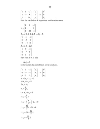
91. 91
 
 
 
 
n n 2
2n
n 2
n
2n 2n
n
2n n 2
n n 2
ar - n r r a .r
r
- n a .r r r
ar
-
r r
n a .r
ar
- r
r r
n a .r
a
- r
r r








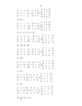
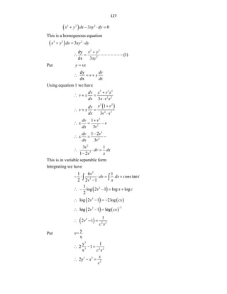
Check your progress:
(1) If ˆ ˆ ˆ
r x i +y j + z k
 and r r

Show that:
a)   2
r
grad log r
r

b) 3
grad r 3 r r

c)    
1 r
grad f r f r
r

(2) If 2 2
= 4x yz + 3xyz 5xyz
 
Find grad  at (3, 2, -1)
(3) Show that 3 5
grad r -3 r r


(4) If   2 2 2
F x, y, z x y + z
  Find F
 at (1, 1, 1)
(5) Show that  
f r r 0
   where ˆ ˆ ˆ
r xi + yj + zk

(6) Find unit vector normal to the surface 2 2 2 2
x y z 3a
   at (a, a, a)
[Hint :- Unit vector normal to surface  i.e.


]
5.3.1 Divergence:
If v (x, y, z) = 1 2 3
ˆ ˆ ˆ
v i + v j + v k can be defined and differentiated at each
point (x, y, z) in a region of space then divergence of v is defined as
div v = . v


92. 92
 
     
1 2 3
1 2 3
ˆ ˆ ˆ
= i j k . v i +v j + v k
x y z
= v v v
x y z
 
  
 
 
  
 
  
 
  
Example 16 If    
2 2 2
ˆ ˆ ˆ
F = x y i + 2xyj + y 2xy k
  , find F
Solution: div F = . F

   
 
     
2 2 2
2 2 2
ˆ ˆ ˆ ˆ ˆ ˆ
= i j k . x y i 2xyj + y 2xy k
x y z
= x y 2xy y 2xy
x y z
= 2x 2x 0
= 4x
 
  
    
 
  
 
  
   
  
 
Example 17 Show that div r = 3 where ˆ ˆ ˆ
r = xi + y j +z k
Solution: div r
 
     
= . F
ˆ ˆ ˆ ˆ ˆ ˆ
= i j k . xi + yj + zk
x y z
= x y z
x y z
= 1 1 1
= 3

 
  
 
 
  
 
  
 
  
 
Example 18 For ˆ ˆ ˆ
r = xi + y j +z k show that  
n n
div r r = (n+3) r
where r r

Solution: L.H.S. div  
n
r r  
n
= . r r

 
     
     
n
n n n
n n 1 n n 1 n n 1
ˆ ˆ ˆ ˆ ˆ ˆ
= i j k . r xi + yj + zk
x y z
= r x r y r z
x y z
r r r
= r 1 + x nr + r 1 + y nr r 1 + z nr
x y z
  
 
  
 
 
  
 
  
 
  
  

  

93. 93
 
 
n n 1
n n 1
2 2 2
n n 1
2
n n 1
n n
n
r r r
= 3r + nr x + y + z
x y z
x y z
= 3r + nr x. y. z.
r r r
x y z
= 3r + nr
r
r
= 3r + nr
r
= 3r + nr
= 3 + n r




 
  

 
  
 
 
 
 
 
 
= R.H.S.
Example 19 Evaluate  
ˆ
div r where ˆ ˆ ˆ
r = xi + y j +z k
Solution: We have n r
r̂ =
r
 
   
2 2
ˆ ˆ ˆ
xi + y j +z k
=
r
ˆ
div r
ˆ
= . r
ˆ ˆ ˆ
xi + yj + zk
ˆ ˆ ˆ
= i j k .
x y z r
x y z
=
x r y r z r
r
r r 1 - y
r 1 - x
y
x
= +
r r


 
 
  
   
   
  
   
  
     
 
     
  
     




 
 
2
2 2 2
2 2 2 2 2 2
3 3 3
2 2 2 2 2 2
3
2 2 2 2
3
r
r 1 - z
z
r
x y z
r - x r - y r - z
r r r
= +
r r r
r - x r - y r - z
= +
r r r
r - x +r - y r - z
=
r
3r - x + y z
=
r



 
 
  




94. 94
2 2
3
3r - r
=
r
2
=
r
Example 20 If 2 3 4
F = x y z Find div (grad F)
Solution: grad F
 
 
     
2 3 4
3 4 2 4 2 3 3
3 4 2 2 4 2 3 3
3 4 2 2 4 2 3 3
= F
ˆ ˆ ˆ
= i j k x y z
x y z
ˆ ˆ ˆ
= 2xy z i + 3y z j + 4x y z k
div (grad F)
ˆ ˆ ˆ
= . 2xy z i + 3y x z j + 4x y z k
= 2xy z + 3y x z + 4 x y z
x y z
=

 
  
 
 
  
 


  
  
3 4 2 4 2 3 2
2xy z + 6x y z + 12 x y z
Example 21 Find the value of div   n
a r r
 where a is a constant
vector and ˆ ˆ ˆ
r = xi + y j +z k
Solution: div   n
a r r

 
 
 
     
 
n
n n
n n 1
ˆ
= i . a r r
x
ˆ
= i . . a r r a r r
x x
r r
ˆ
= i . a r a r n r
x x
a
x




 
 
 
  
 
 
 
 
 
 
 
 
  
 
 
 
 
 




   
   
    
 
n n 1
n n 2
n 2
n 2
0
x
ˆ ˆ
= i . a i r a r n r
r
ˆ ˆ
= i . a i r nx r a r
ˆ ˆ ˆ
= nr x i a r i. a i = 0
ˆ
nr a r x i




 

 
 
 
  
 
 
 
  
 
 
 
 
 





95. 95
 
 
 
n 2
n 2
n 2
ˆ
nr a r r xi r
nr a r . r
nr 0
0



 
  
 
 
 
 



5.3.4 Solenoidal Function: A vector function F is called Solenoidal if
div F = 0 at all points of the function.
5.3.5 Curl: The curl of a vector point function F is defined as curl
F F
  if 1 2 3
ˆ ˆ ˆ
Fi + F j +F k .
 
 
1 2 3
curl F F
F
ˆ ˆ ˆ ˆ ˆ ˆ
= i j k Fi + F j +F k
x y z
  
  
 
  
  
 
  
 
1 2 3
3 3
2 1 2 1
ˆ ˆ ˆ
i j k
=
x y z
F F F
F F
F F F F
ˆ ˆ ˆ
= i - j + k
y z x z x y
  
  
   
 
   
 
  
   
 
     
 
   
The curl of the linear velocity of any particle of rigid body is equal to
twice the angular velocity of body.
i.e. if 1 2 3
ˆ ˆ ˆ
w = w i + w j +w k be the angular velocity of any particle of the
body with position vector defined as ˆ ˆ ˆ
r = xi + yj +zk then linear velocity
v = w r
 .
Hence curl v v
  
 
     
1 2 3
2 3 1 3 1 2
= w r
ˆ ˆ ˆ
i j k
= w w w
x y z
ˆ ˆ ˆ
= i w z -w y j w z -w x k w y -w x
  
 
 
   
 

96. 96
     
2 3 3 1 1 2
1 1 2 2 3 3
1 2 3
ˆ ˆ ˆ
i j k
=
x y z
w z -w y w x -w z w y -w x
ˆ ˆ ˆ
= i w + w j w -w k w + w
ˆ ˆ ˆ
= 2w i 2w j 2w k
= 2w
curl v = 2w
  
 
  
  
 

5.3.6 Irrotational field:
A vector point function F is called irrotational if F 0
 at all points of the
function.
Example 22 Find curl (curl F) If 2 ˆ ˆ ˆ
F = x y i -2 x z j 2 y z k
 at (1, 0, 2)
Solution: Curl F
   
   
       
 
2
2
2
2
2 2
ˆ ˆ ˆ
i j k
=
x y z
x y 2xy 2yz
ˆ ˆ
= 2z +2x i 2z -x k
ˆ
curl curl (F) = 2z + 2x i + 0j + 2z x k
ˆ ˆ ˆ
i j k
=
x y z
2z +2x 0 2z x
ˆ ˆ
= i 2z x 0 j 2z x 2z 2x
y z x z
ˆ
k 0
x
  
  

 
 
    
 
  
  
 
 
   
 
       
   
   
 
 
 
 
 
 
     
 
2z 2x
y
ˆ ˆ ˆ
= i 0 j 2x 2 k 0
ˆ
= 2x 2 j
 

 
 
   

At (1, 0, 2)

97. 97
    ˆ
curl F 2(1) + 2 j
ˆ
4 j


Example 23 Find curl V if      
2 2 2
ˆ ˆ ˆ
V = x + yz i + y +2x j z +xy k
Solution: curl V
       
2 2 2
2 2 2 2
V
ˆ ˆ ˆ
i j k
=
x y z
x yz y zx z xy
ˆ ˆ
i z +xy y +2x - j z +xy y +yz
y z x z
  
  
  
  
 
   
 
  
   
   
 
 
   
2 2
ˆ
+ k y +2x x + yz
x y
 
 

 
 
 
     
ˆ ˆ ˆ
i x - x - j y - y + k z - z
0


Example 24 Evaluate curl r where if ˆ ˆ ˆ
r = xi + yj zk

Solution: Curl r
ˆ ˆ ˆ
i j k
=
x y z
x y z
z y z x y x
ˆ ˆ ˆ
i - j + k
y z x z x y
ˆ ˆ ˆ
0i - 0j+ 0k
0
  
  
   
     
 
   
   
 
     
 
   


Example 25 Evaluate curl
r̂
r
 
 
 
where if ˆ ˆ ˆ
r = xi + yj zk

Solution:
2
2 2 2
r
r̂ =
r
r̂ x y z
ˆ ˆ ˆ
= i j k
r r r r
 
 
 
  

98. 98
2 2 2
2 2 2
2 2 2 2
2 2
3
r̂ x y z
ˆ ˆ ˆ
curl = i j k
r r r r
ˆ ˆ ˆ
i j k
x y z
x y z
r r r
z y z x
ˆ ˆ
i - j
y r z r x r z r
y x
ˆ
+ k
x r y r
2z
î
r
   
    
   
   
  

  
   
   
       
  
       
   
   
       
 
 
 
 
   

   
 
 
   
 

 3
3 3
3 3 3
2r 2y 2r
+ + -------------+---------------
2y r 2z
2z y 2y z
î + + -------------+---------------
r r r r
2yz 2yz 2zx 2zx 2xy 2xy
ˆ ˆ ˆ
i + j + k
r r r
ˆ ˆ ˆ
= 0i + 0j + 0k
 
 
 

 
  
 
 
  
     
      
 
     
 
 0
Example 25 If 2 ˆ ˆ ˆ
F = x y i + xzj 2yzk
 find div (curl F)
Solution: curl F
       
   
     
   
2
2
2
2
2
ˆ ˆ ˆ
i j k
x y z
x y xz 2yz
ˆ ˆ
i 2yz xz - j 2yz x z
y z x z
ˆ
+ k x z x z
x y
ˆ ˆ ˆ
i 2z - x - j 0 - 0 + k z - x
ˆ ˆ
2z - x i + z - x k
div (curl F)
  

  
 
   
 
  
   
   
 
 
 
 

 
 
 



99. 99
   
   
2
2
ˆ ˆ ˆ ˆ ˆ
i j + k . 2z - x i z x k
x y z
2z - x z x
x z
= 1 + 1
0
 
    
   
   
  
 
 
  
 


Example 27 If  
F = grad xy + yz zx
 , find (curl F).
Solution:  
F = grad xy + yz zx

 
 
     
     
xy + yz +zx
ˆ ˆ
i j + k xy + yz +zx
x y z
ˆ ˆ ˆ
i xy + yz +zx + j xy + yz +zx + k xy + yz +zx
x y z
ˆ ˆ ˆ
i y + z + j x z + k y + x
(curl F)
ˆ ˆ ˆ
i j k
x y z
y z x + z x + y
 
 
  
 
 
  
 
  

  
 

  

  

       
   
     
ˆ ˆ
i x + y - x + z - j x + y y + z
y z x z
ˆ
+ k x + z y + z
x y
ˆ ˆ ˆ
i 1 - 1 - j 1 - 1 + k 1 - 1
ˆ ˆ ˆ
0 i + 0 j + 0 k
0
 
   
 
 
   
   
 
 
 
 

 
 
 



5.4 PROPERTIES OF GRADIENT, DIVERGENCE AND
CURL
(i)  
f g = f g
    
(ii)  
. A B = . A . B
    
(iii)  
A B = A . B
     

100. 100
Proof:
(i)  
f g
   
ˆ ˆ ˆ
i + j + k f g
x y z
 
  
 
 
  
 
     
ˆ ˆ ˆ
i f g j f g + k f g
x y z
ˆ ˆ ˆ ˆ ˆ
i f + j f + k i g+ j g + g
x y z x y z
f g
  
    
  
   
     
 
   
     
   
   
(ii) Let 1 2 3
ˆ ˆ ˆ
A = A i + A j +A k
 
     
     
           
1 2 3
1 1 2 2 3 3
1 1 2 2 3 3
1 2 3 1 2 3
ˆ ˆ ˆ
B = B i + B j +B k
. A B
ˆ ˆ ˆ
. A B i A B j A B k
A B + A B + A B
x y z
A + A + A B + B + B
x y z x y z
. A . B
  
 
      
 
  
   
  
 
     
   
     
 
   
(ii) Let
 
   
 
1 1 2 2 3 3
3 3 2 2
A B
ˆ ˆ ˆ
i j k
x y z
A B A B A B
ˆ
i A B A B
y z
ˆ
i A B
x
A B
ˆ
i
x x
A B
ˆ ˆ
i i
x x
A B
  
  

  
  
 
 
   
 
 
 

  

 
 
  
 
 
 
 
   
 
   



 

101. 101
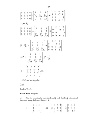
Check Your Progress:
(1) If 1 2 3
ˆ ˆ ˆ
A = A i + A j +A k , ˆ ˆ ˆ
r = x i + y j + z k Evaluate  
div A r

(2) Prove that
 
log r 1
div r 1 2 log r
r r
 
 
 
 
(3) For ˆ ˆ ˆ
r = x i + y j + z k ) show that the vector 3
r
div
r
 
 
 
is both
solenoidal and irrotational.
(4) Prove that  
2
div a. r a = a
(5) For ˆ ˆ ˆ
r = x i + y j + z k show that    
n n 2
. r = n n 1 r 
  
(6) show that the vector ˆ ˆ ˆ
F = yzi + zxj + xyk solenoidal.
(7) If      
ˆ ˆ ˆ
A = ax + 3y +4z i + x - 2y +3z j + 3x + 2y - z k is
solenoidal find value of a.
(7) Find the direction derivative of a scalar field 2
x y z
  at (4, -1, 2)
in the direction of (3, 2, 1).
[Hint :- direction derivative of  (x, y, z) along a is = a . grad  ]
5.4 PROPERTIES OF GRADIENT, DIVERGENCE AND
CURL
1) If S represents displacement vector,
ds
dt
represents velocity and
2
2
d s
dt
represents acceleration.
2) For
ds ˆ ˆ ˆ
i j k
dt x y z
  
   
  
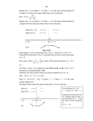
grad f F
grad F . F
curl F F
 
 
  
3) grad F and curl F are vector quantities.
4) div F is scalar quantity.

102. 102
5.5 LET US SUM UP
In this chapter we have learn
 Differentiation of vectors.
 Partial derivative of vectors.
 The vector differential Operator Del.(  )
 Divergence of a vector function.
 Curl of a vector.
 Properties of divergence, gradient & curl.
5.6 UNIT END EXERCISE
1) If 2 2
A x yi 2xzj xy k,
   2
B 3zi 2yj 2x k
  
Find the value
2
(A B)G (1,0,1)
y x

 
 
2) If r xi yi zk
   prove that 3
1 1
r.
R R

 

 
 
where R r

3) Find the unit normal vector to the surface at the point(1,0,1).
4) Find the directional derivative of 2 3
f(x,y,z) xy yz
  the point
(1,-1,1) in the direction of (3,-1,1)
5) If 2 2
f 3x y xyj 3y zk
   find div F curl F.
6) Show that the vector f (x 3y)i (y 3z)j (x 2z)k
      is
solenoid.
7) Show that the vector 2 3 2 2 2
f (3x y)i (x 2yz )j (3z 2y z)k
     is
irrotational.
8) Show that div r =3
where r xi yi zk
  
9) Show that for any vector F
Div (Curl F)=0
10) If 1 2 3
a a i a i a k
   and r xi yj zk
  
Find Curl (r x a)
*****

103. 103
6
DIFFERENTIAL EQUATIONS
UNIT STRUCTURE
6.1 Objective
6.2 Introduction
6.3 Differential Equation
6.4 Formation of differential equation
6.5 Let Us Sum Up
6.6 Unit End Exercise
6.1 OBJECTIVE
After going through this chapter you will able to
i. Define differential equation
ii. Order & degree of differential
equation
iii. Formulate the differential equation
6.2 INTRODUCTION
We have already learned differential equation in XIIth . Hence we
are going to discuss differential equation in brief. In this chapter we
discuss only formulation of differential equation.
6.3 DIFFERENTIAL EQUATION
Definition:-
An equation involving independent and dependent variables and the
differential coefficients or differentials is called a differential equation.
e.g. 1
dy
=9
dx
x=independent variable
y= depedent variable
2
2
2
d y
2 +y=0
dx
dy
dx

3
n
n
d y
y=0
dx


104. 104
These are all examples of differential equations.
The differential equation is said to be ordinary if it contains only one
independent variable. All the examples of above are of ordinary
differential equations.
Order and Degree of a Differential Equations:-
(i) Order:-
The order of the differential equations is the order of the highest orderal
derivatives present in the function or equation.
If y = f (x) is a function, then
dy
dx
is the first order derivative,
2
2
d y
dx
d dy
dx dx
 
  
 
is the second order derivative.
e.g 1)
2
2
d y
2 0
dx
dy
y
dx
  
Order = 2
2) E = Ri + L
di
dt
Order = 1
Degree:-
The degree of differential equation is the degree of the highest ordered
derivative in the equation when it is made free from radicals and fractions.
e.g.
1
2
2
2
d y
0
dx
k y
 
order = 2, degree = 1
2
2
2
2
d y
2 0
dx
dy
Y
dx
 
  
 
 
Order =2, degree =1
3
1
dy
y x
dy
dx
dx
 
 
 
 
Order=1, degree=2
4
2
3
2
dy
dx
dy
dx

1 1
2 3 2
2
d y dy
dx dx
   
 
   
 
 
Cubing both sides

105. 105
3 2
2
2
dy
dx
y
d
dx
 
   
 
Squaring both sides
2 3
2
2
dy
dx
y
d
dx
   
 
   
 
 
Order=2, degree=2
Solved examples:
Example 1: Find the order and degree of the following
3
2 2
2
2
1
i)
dy
dx
e
d y
dx
 
 

 
 
 
 
 

Solution:
3
2 2
2
2
e 1
d y dy
dx dx
 
 
   
 
 
 
 
 
Squaring both sides
3
2 2
2
2
2
e 1
d y dy
dx dx
 
   
  
 
   
 
 
   
 order = 2, degree = 2
ii)
3
2
3
sin( ) x
d d y
x xy e
dx dx
 
 
 
 
 
 
 
 
 
Solution:
3 2
3 3 4
3 3 4
d
x 3 sin( )
y
x
d y d y
xy e
dx dx dx
   
    
   
   
 Order = 4, degree=1
iii)
5
dy
y x
dy
dx
dx
  
Solution:
2
dy
y 5
dy
x
dx dx
 
    
 
 
 Order =1, degree=2

106. 106
iv)
2
5 1
dy dy
y x
dx dx
 
    
 
Solution:
2
dy
y x 5 1
dy
dx dx
 
      
 
Squaring on both sides
2 2
dy
y-x 25 1
dx
dy
dx
 
   
  
 
   
   
 
 
2 2
2 2
y 2 25 1
dy dy dy
xy x
dx dx dx
 
   
     
 
   
   
 
 
 Order =1, degree=2
Check your progress:
1)
2
2
u u
u
x y
 
 
 
Ans : order =2, degree=1
2)
4 7 11
3 3 2
3 3 2
5 7 x
d y d y d y dy
y e
dx dx dx dx
     
    
     
     
Ans : order=3, degree=7
3)    
3 4
11 1 x
y y e
 
Ans : order=2, degree=3
4) 11
11
1
x
y
y
 
Ans : order=2, degree=2
5) 11 12
1
y y
 
Ans : order=2, degree=2
 
2
1 1
y x y xy

  
Ans : order =1, degree=3
6.4 FORMATION OF DIFFERENTIAL EQUATION
Formation of differential equation involves elimination of arbitrary
consonants, in the relation of the variables.
Consider

107. 107
2
1
y ax
 
Where y= independent variable
x = dependent variable
Differentiating equation (1) with respect to x
we have
dy
2 (2)
dx
ax
           
From equation (1) we have
2
y
a
x

Put value of a in equation (2), we have
2
dy
2
y
x
dx x
    
dy 2
dx
y
x
 
dy
x 2
dx
y
  
dy
x 2 0
dx
y
   
This is the required differential equation
Note:-
To eliminate two arbitrary constants, three equations are required. To
eliminate three arbitrary constants, four equations are required.
In general to eliminate n arbitrary constants. (n+1) equations are required.
In other words elimination of n arbitrary consonants will bring us to
differential equation of nth order.
Solved Examples:-
Example 2: Form the differential equations if 1 2
cos sin
y c x c x
 
Solution: We have
Y= c1 cos x + c 2 sinx -------------(1)
This equation contains two arbitrary constants, therefore we shall require
three equations to eliminate c1 and c 2 .
Differentiating equation (1) with respect to x
1 2
dy
= -c cos cos .
dx
x c x
 
Again differentiate with respect to x
2
1 2
2
d
= -c cos sin
dx
y
x c x
 

108. 108
2
1 2
2
d
= (c cos +c sin )
y
x x
dx

 
2
2
d
= ----(1)
y
y from eq
dx
          
2
2
d
+ y = 0
dx
y

This is the required differential equation.
Example 3: Form the differential equation from
x= a sin (wt+c) where a and c are arbitrary constants.
Solution: We have,
x= a sin (wt+c)--------(1)
Differentiate equation (1) with respect
dx
+ acos (cot+c) w
dt
  
dx
+ aw cos(cot+c)
dt
  
Again differentiating w.r.t. 't'
 
2
2
d x
-a wsin cot c w
dt
  
 
2
2
2
d x
-w a sin cot c
dt
 
 
 
 
2
2
2
d x
- ........ sin equation 1
w x u g
dt
 
2
2
2
d x
w x 0
dt
  
This is the required differential equation
Example 4: From the differential equation if y= log (ax)
Solution:
log( ) (1)
y ax
 
Differentiate equation (1) with respect to x .
dy 1
dx
A
Ax

  

dy 1
dx x
 
dy
x 1
dx
  
This is the required differential equation.

109. 109
Example 5: Obtain the differential equation for the equation Y=cx+ c2
Solution: we have,
2
(1)
y cx c
  
Differentiate equation (1) with repect to x
dy
dx
c
 
Put value of c in equation (1)
2
dy dy
y= x
dx dx
 
    
 
This is the required differential equation.
Example 6: Obtain the differential equation for the relation
2x 3
y= a e a,b are constants.
x
b e Where
   
Solution: we have,
2x 3
y= a e -------------(1).
x
b e
    
Here the number of arbitrary constants is two
Hence we shall require three equations to
Eliminate and b. So we differentiate the given equations twice.
2x 3
dy
= 2a e 3 -------------(2).
dx
x
b e
    
2
2x 3
2
d y
= 4a e 9 -------------(3)
dx
x
b e
    
From equation (1) (2) & (3) elimination of a & b gives directly
2
2
1 1
dy
2 3 0
dx
4 9
y
d y
dx

In the determinant
1st column is LHS
Column 2nd column 2nd column contains coefficients 2x
a e

Expanding the determinant
2nd column contains coefficients of 3x
b e

     
2
2
18 12 9 4 3 2 0
dy d y
y
dx dx
      
2
2
dy d y
6y-5 0
dx dx
   

110. 110
2
2
d y dy
-5 +6y 0
dx dx
  
This is the required differential equation.
Example 7: Find the differential equation of all circles
touching y axis at the origin and centers on x-axis
Solution:
The equation of such a circle is
 
2 2 2
x a y a
  
i.e. 2 2 2 2
2
x ax a y a
 
   
 
2 2
2 0 (1)
x y ax
    
Where a is the only arbitrary contents
Differentiate equation (1) with respect to x We have
2 2 2 0
dy
x y a
dx
   
2 2
x 2 0
dy
y x x y
dx
 
     
 
 
2 2 2
x 2 2 0
dy
y x xy
dx
    
2 2
-x 2 0
dy
y xy
dx
   

111. 111
2 2
2 x 0
dy
xy y
dx
    
Which is the require differential equation.
Check Your Progress:
1) Form the differential equation of all circles of radius a.
Ans.
3
2 2
2
2
1
dy d y
a
dx dx
   
 
 
   
 
 
   
 
2) Obtain the differential equation whose general solution is given by
 
cos sin
x
y e A x B x
 
Ans
2
2
2 2 0
d y dy
y
dx dx
  
3) Find the differential equation whose general solution is given by
2 3
1 2 3
x x x
y c e c e c e


   
Ans
3 2
3 2
2 5 6 0
d y d y d y
y
d x d x d x
    
4) Obtain the differential equations for the following:
i) 3 2
x x
y A e B e
   
Ans
2
2
5 6 0
d y dy
y
dx dx
   
ii) 2
1 2
t t
s c e c e
  
Ans
2
2
2 0
d s ds
s
dt dt
  
iii) cos 2t+ B sin 2t
y A

Ans
2
2
d
4 0
y
y
dt
 
iv) 3 2
y ax bx
 
Ans
2
2
2
4 6
d y dy
x x y o
dx dx
   
v) cos(
x A nt 
 
Ams
2
2
2
0
d y
n x
dt
 
vi 2
Y A Bx Cx
  
Soln
2
2
0
d y
dx

Vii sin
Y x c
 

112. 112
Soln cos
dy
x
dx

Viii 1 2
( ) x
y c c x e
 
Ans
2
2
2 0
d y dy
y
dx dx
   
6.5 LET US SUM UP
In this chapter we have learn
 Equation in term
dy
dx
of is called differential equation.
 Degree & order of differential equation.
 Formation of differential equation while removing arbitrary
constant likes A&B,&C.
6.6 UNIT END EXERCISE
1) Find the order 7 degree of Differential equation given below
i.
2
3 2
3 2
3 3
d y d y dy
y
dx dx dx
   
  
   
   
ii.
3
2 2 2
2
dy d y
i k
dx dx
 
 
 
 
 
 
 
 
iii.
3
2 5
2
1
d y dy
dx dx
   
 
   
 
 
iv.
2
2
3
2
2 1 0
d y dy
y
dx dx
 
   
 
 
v.
 
1
dy
y x
dy
dx
dx
 
 
 
 
2) Formulate the differential equation
i. Y A Blogx
 
ii. X = asin(w++c)
iii. x
Y = c (Acosx+Bsinx)
iv.
1
cos
m x
Y = e

v. 2
Y = ax bx

vi. 2 3
Y = cx+2c c

vii. 2 2
X +Y = 2ax
viii. 2
Y = 4ax
ix. x y
e +Ce =1

113. 113
x. Y = ACos2x+BSin2x
*****
7
SOLUTION OF DIFFERENTIAL
EQUATION
UNIT STRUCTURE
7.1 Objectives
7.2 Introduction
7.3 Solution of Differential equation
7.4 Solution of Differential Equation of first order and first degree
7.5 Let Us Sum Up
7.6 Unit End Exercise
7.1 OBJECTIVES
After going through this chapter you will able to
 Find general & particular solution of differential equations.
 Classification of differential equation.
 Apply particular method first find the solution of differential
equation.
7.2 INTRODUCTION
We have already formed differential equation in previous chapter.
Here we are going to find solution of differential equation with different
method. It is very useful in different field.
7.3 SOLUTION OF DIFFERENTIAL EQUATION
General Solutions:-
The general Solution of a differential equation is the most general
relation between the dependent and the independent variable occurring in
the equation which satisfies the given differential equation.
Particular Solutions:-

114. 114
Any particular solution that satisfies the given equation is called a
particular solution e.g.
5
dy
dx

dy=5dx

Integrating both sides we get
dy=5 dx constant
  
 
Y= 5x+C
This is called as general solution
Suppose C=7 is given
Then particular solution is given by putting of c in the general solution
y = 5x+7

Check Point:-
1) Find the general solution and particular solution of the differential
equation
When y 4 at x 0
dy
x
dx
  
Solution:
2
x
=
2
y c

2
x 4
2
y  
Differential equations of first order and of First Degree :-
An equation of the form,
M+N 0
dy
dx

Where „M‟ and „N‟ are functions of x and y or constant. is called
differential equation of first order and first degree.
This equation can also be written as
0
Mdx Ndy
 
7.4 SOLUTION OF DIFFERENTIAL EQUATION OF
FIRST ORDER AND FIRST DEGREE
There are many methods that can be used to solve the differential
equations. Important one among those are listed below.
1) Variable seperable form.
2) Equations reducible to variable seperable form.
3) Homogeneous equations.
4) Exact differential equations.
5) linear differential equations.
6) Equations reducible to linear differential equation.( Bernoullis‟s
differential equation)

115. 115
7) Methods of substitution.
We will explain all these methods one by one in detail.
7.4.1 Variable Separable form:-
Working Rule
1) Consider the differential equation Mdx+ Ndy=0
2) If possible rearrange the terms and get f(x) dx +g(y).dy=0
3) Integrate and write constant of integration in suitable form, usually
C.
4) Simplify if possible.
Solved Examples:-
Example 1: Solve     2
3 tan 1 . 0
x x
y dx e Sec y dy
   
Solution:     2
3 tan 1 . 0
x x
y dx e Sec y dy
   
 
x
throughout by 1-e tan we get
y
 
x 2
x
3e sec
0 1)
1-e tan
y
dx dy
y
 
          
 
 
This is in variable separable form
 Integrate equation (1), we get
2
3
1 tan
x
x
e Sec y
dx dy constant
e y
  
 
2
x
e
-3
e 1 tan
Sec y
dx dy c
y
    

 
 
x
-3log e 1 log tan log
y c
   
 
3
x
log e 1 log tan log
y c

   
 
-3
x
log e -1 ×tany = logc

 
3
x
tany
= c
e -1

Removing log both side
 
3
x
tany = c× e -1

This is the general solution of a given differential equation.
Example 2: Solve 2 2 2 2
1
y dy
x y x y
x dx
    

116. 116
Solution:  
2 2 2
1 1
y dy
x y x
x dx
    
   
2 2
y dy
× = 1+x × 1+ y
x dx
   
2 2
y dy
× = 1+x × 1+ y
x dx
 
 
2
2
y
×dy = x 1+ x ×dx ----------1
1+ y

This is in variable separable form
 Integrate equation (1)
2
2
1 2 1
2 1
2 2
1
y
dy x x dx c
y
       

 
 
 
 
   
 
1
n
1
n+1
f x
dx= 2 f x +c
f x
f x × f x dx
f x
=
n+1





 
  

  
 





 
3
2 2 2
1 1 2
× 2 1+ y = × × 1+ x +c
2 2 3
 
 
  
   
 
3
2 2 2
1
1+ y = 1+ x +c
3
This is in required general solution.
Example 3: Solve  
1 1 2 y
dy
x e
dx

   
Solution: The given equation is
   
1 2 1
y
dy
x e
dx

    
 
-y
1 1
×dy = ×dx
x+1
2e -1

 
y
y -y
e 1 1
× ×dy = ×dx
e x+1
2×e -1

1
2 1
y
y
e
dy dx
e x
   
 
1
0=
x+1 2
y
y
e
dx dy
e
   


117. 117
2
1
0 (1)
1
y
y
e
dx dy
x e 
         

This is in variable separable form,
Integrate equation (1), we get
 
1
=log c
1 2
y
y
e
dx dy
x e
 
 
 
   
log 1 log 2 log
y
x e c
    
   
log x+1 2 log
y
e c
 
   
 
   
1 2
y
x e c
    
This is the required general solution.
Example 4: Solve   2
3 tan 1 sec 0
x x
e y dx e y dy
    
given
4
y

 when x=0
Solution: The given equation is
  2
3 tan 1 sec 0
x x
e y dx e y dy
    
 
x
through out by 1+e tan y
 
x 2
x
3e sec
0 (1)
1+e tan
y
dx dy
y
              
This is in variable separable form,
Integrate equation (1) we get
x 2
x
3e sec
log
1+e tan
y
dx dy c
y
    
 
x 2
x
e sec
3 log
1+e tan
y
dx dy c
y
     
 
 
3log 1 log tany=log c
x
e
 
 
3
x
log 1+e log tany=log c
 
 
3
x
log 1+e tan log
y c
 
  
 
 
 
 
3
x
1+e tan =c---------------(2)
y
 
This is the required general solution
To final particular solution:-
put y= at x=0 in equation --------(2)
4


118. 118
 
3
1+1 tan
4
c

  
c=8

Put value of c in equation (2)
 
3
1 tan 8
x
e y
   
This is a particular solution
Example 5: Solve
 
2log x 1
sin y y cos y
x
dy
dx



Solution: The given equation is
 
2log 1
sin cos
x x
dy
dx y y y



   
sin cos 2log 1 (1)
y y y dy x x dx
      
This is in variable separable form
Integrate equation (1), we get
   
sin cos 2log 1 tan
y y y dy x x dx cons t
     
 
siny cos 2 log
dy y y dy x x dx xdx c
         
   
2 2 2
cos sin cos 2 log
2 2 2
x x x
y y y y x c
 
        
 
 
2 2 2
sin log
y y x x x x c
   
2
sin log
y y x x c
  
This is required general solution
Check Your Progress:
1) solve:
2
x y y
dy
e x e
dx
 
  
3
3
x y
x
e e c
  
2) solve: 2
dy dy
y x a y
dx dx
   
    
   
   
ans   
1 ay x a cy
  
3) solve: log
dy
ax by
dx
 
ans
ax by
e e
c
a b

 
4) solve: cos cos sin 0
dy
x x y y
dx
  
ans sin cos logcos
x x x y c
  

119. 119
5) solve: 2 2
tan sec tan 0
Sec x y dx y x dy
     
ans tan tan
x y c
 
6) solve: 2
x y
dy
e
dx


ans 2
1
2
y x
e e c
  
7.4.2 Equations Reducible to variable separable forms:
Sometimes we come across differential equations which cannot be
converted into variable separable form by mere rearrangement of its terms.
These differential equation can be suitable substitution
Solved Examples:-
Example 6: solve:  
2 2
dy
x y a
dx
  
Solution: we have  
2 2
(1)
dy
x y a
dx
            
Substitute x-y=t
Differentiating with respect to x, we get
1
dy dt
dx dx
 
1
dy dt
dx dx
  
Using equation (1) we have
2 2
t 1
dt
a
dx
 
  
 
 
2
2
1
dt a
dx t
  
2
2
1
dt a
dx t
  
2 2
2
dt t a
dx t

 
2
2 2
t
dt dx
t a
  

This is invariable separable form
Integrating we get
2
2 2
tan
t
dx dt cons t
t a
  

 
2 2 2
2 2
x=
t a a
dt c
t a
 
  



120. 120
2
2 2
x=
a
dt dt c
t a
   

 
2 1
x=t+ log
2
t a
a c
a t a

 
   
  

 

a
x=t+ log
2
t a
c
t a

 
  
 

 
t=x-y
a
x=x-y+ log
2
x y a
c
x y a
 
 
  
 
 
 
a
y= log
2
x y a
c
x y a
 
 
 
 
 
 
This is the required general solution
Example 7: Solve  
cos
dy
x y
dx
 
Solution: We have  
cos (1)
dy
x y
dx
          
Put x y t
 
Differentiating above with respect to x, we get
1+
dy dt
dx dx
 
1
dy dt
dx dx
  
Using equation (1)
1 cos
dt
t
dx
  
1 cos
dt
t
dx
  
1
1 cos
dt dx
t
  

2
1
2cos
2
dt dx
t
 
This is invariable separable form,
Integrating we get
2
1
tan
2cos
2
dt dx cons t
t
   
 
2
1
sec
2
2
t dt x c
    


121. 121
1 2
tan
2
2 1
t x c

    

tan
2
t x c
  
t=x+y
tan
2
x y
x c

 
  
 
 
This is the required general solution,
Example 8: Solve  
2
4 1
dx
x y
dy
  
Solution: The given equation is  
2
dy
4 (1)
dx
x y
       
Put  
4x y t
 
Differentiating above with respect to x
4
dy dt
dx dx
  
4
dy dt
dx dx
  
Using equation (1), we have
2
4
dt
t
dx
 
2
4
dt
t
dx
  
2
1
4
dt dx
t
  

This is in variable separable form
Integrating we get,
2
1
tan
4
dt dx cons t
t
   

 
1
1
tan
2 2
t
x c
  
   
 
 

t=x+y
1
1
tan
2 2
x y
x c
 
 
   
 
 
1
1 1
tan 2 where c
2
x y
x c c
 
 
   
 
 
This is the required general solution
Example 9: Solve  0
dy
x y y
dx
   

122. 122
Solution:
  0 (1)
dy
x y y
dx
             
Put x y t
 
Differentiating with respect to x, we get
dy
1+
dx
dt
dx
 
dy
1
dx
dt
dx
  
Using equation (1), we have
t 1 0
dt
t x
dx
 
     
 
 
1
dt x t
dx t

 
1 1
dt x
dx t
 
   
dt x
dx t
 
xdx tdt

This is in variable separable form
Integrating we get,
xdx= tdt+constant
 
2 2
2 2
x t
c
 
2 2
x 2
t c
  
t=x+y
 
2
2
x 2
x y c
   
2 2 2
x 2 2
x xy y c
    
2
2xy 2
y c
   
2
1 1
2xy where c 2
y c c
    
This is the required general solution
Example 10: Solve cos sin cos 0
y y x y y
dx dy
x x y x x
 
 
     
 
 
   
Solution:
The equation is, cos sin cos 0
y y x y y
dx dy
x x y x x
 
 
     
 
 
   

123. 123
Substitute
y
v
x

y=vx

Differentiating above with respect to x, we get
dy
dx
dv
v x
dx
   
But the above equation can be written as
y
cos sin cos 0
x
y x y y dy
x y x x dx
 
      
 
 
1
v cosv- sin cos 0
v
dy
v v v x
dx
   
      
   
   
By rearranging the terms, we have
1 sin cos
x sin
v v v
dx dv
v v

   
1 sin cos
0
x sin
v v v
dx dv
v v

   
This is in variable separable form
Integrating we get,
1 sin cos
tan
x sin
v v v
dx dv cons t
v v

    
 
 
logx+log vsinv c
 
 
log x vsinv logc
 
 
xv sinv=c

y
v=
x
y y
x sin
x x
c
  
y
ysin
x
c
 
This is the required general solution
Check Your Progress:
Solve the following
1)
-y
x
Ans : log cx=e
y
x
dy y
e
dx x
 
2) 1 1 0 Ans : x+y e
x x x
y y y
x dy
e e c
y dx
 
 
      
   
   

124. 124
3)   2 2
2 0 Ans:y 2
y y y
x x x
dy
x y e y x e x e c
dx
 
        
 
 
2 2
tan sec sec 0
y y y y
dx dy
x x x x
 
    
 
 
Ans tan
y
x c
x
 
 
 
 
7.4.3 Homogeneous Equations
A differential equation Mdx+Ndy=0 is said to be homogeneous if M & N
are homogeneous functions of x and y of same degree
Working Rule:
1) Check whether differential equation is homogenous in x and y
2) Express
dy
dx
in terms of x and y
3) Put y=vx
4)
dy dv
v x
dx dx
   
5) Separate x and y variables and get F(ex)dx+ g(v) dv=0
6) Solve by integration
7) Put
y
v =
x
and simplify
Solved examples:-
Example 11: Solve
 
2 2
2 0
x y dx xy dy
   
Solution: We have
 
2 2
2 0
x y dx xy dy
   
Here M and N are homogeneous expressions in x and y of the second
degree
 
2 2
2xy dy=- x y dx
  
 
2 2
2xy dy=- x y dx
  
2 2
dy
(1)
dx 2
x y
xy
 

             
 
 
y=vx
put
dy
dx
dv
v x
dx
   
Using equation 1 we have
2 2 2
2
dv x v x
v x
dx x vx

 
 

125. 125
 
2 2
2
1
2
x v
dv
v x
dx v x


  
  
2
dv 1 2
x 1
dx 2
v
v

  

2
dv 1 3
x
dx 2
v
v

 

2
-2v 1
1+3v
dv dx
x
  
This is in variable separable form
Integrating above expression we have
2
1 6v 1
- dv= tan
3 1+3v x
dx cons t
  
 
 
2
1
- log 1+3v log log
3
x c
  
   
2
1
- log 1+3v log
3
cx
 
   
2
log 1+3v 3log cx
  
   
3
2
log 1+3v 3log cx

  
 
2
3 3
1
1+3v
c x
 
y
v
x

2
2 3 3
y 1
1+3
x c x
  
3 2
3
1
x 3xy
c
  
3 2
3
1
x 3 where k=
c
xy k
  
This is the required general solution
Example 12: Solve 2 2 dy dy
y x xy
dx dx
   
Solution:
The given equation is 2 2 dy dy
y x xy
dx dx
   
2 2
dy dy
y xy x
dx dx
    
 
2 2
dy
y xy x
dx
  

126. 126
2
2
(1)
dy y
dx xy x
         

This is a homogeneous equation
Put y=vx
dy dv
v x
dx dx
   
Using equation (1),we have
2 2
2
dv v x
v x
dx x vx x
   
 
 
2 2
2
1
dv v x
v x
dx x v

   


 
2
1
dv v
x v
dx v
   

 
1
dv v
x
dx v
  

1 1
v
dv dx
v x

   
1 1
1 dv dx
v x
 
  
 
 
This is in variable separable form
Integrating we get,
1 1
1 dv = tan
x
dx cons t
v
 
 
 
 
 
vlogv=logx+logc

v=logv+logx+logc

 
v=log vxc

y
v=
x
y y
=log
x x
x c
 
  

 

 
y
=log y
x
c

y=xlog y
c

This is the required general solution
Example 13: solve  
3 3 2
3 0
x y dx xy dy
   
.
Solution:

127. 127
 
3 3 2
3 0
x y dx xy dy
   
This is a homogenous equation
 
3 3 2
3
x y dx xy dy
  
3 3
2
dy
(1)
dx 3
x y
xy

        
Put y vx

dy
dx
dv
v x
dx
  
Using equation 1 we have
3 3 3
2 2
3
dv x v x
v x
dx x v x

  

 
3 3
2 3
1
3
x v
dv
v x
dx v x

  

3
2
1
3
dv v
x v
dx v

  
3
2
1 2
3
dv v
x
dx v

  
2
3
3 1
1 2
v
dv dx
v x
  

This is in variable separable form
Integrating we have
2
3
1 6 1
tan
2 2 1
v
dv dx cons t
v x
    

 
 
3
1
log 2 1 log log
2
v x c
    
   
3
log 2 1 2log
v cx
   
   
2
3
log 2 1 log
v cx

  
 
 
 
3
2 2
1
2 1
v
c x
  
Put
y
v=
x
3
3 2 2
y 1
2 1
x c x
  
3 3
2
2y
x
x
c
  

128. 128
3 3
2
1
2y where k=
c
x kx
  
This is the required general solution
Example 14: solve 2 2
tan sec sec 0
y y y
x y dx x dy
x x x
 
   
 
 
Solution:
The given equation is
2 2
tan sec sec 0
y y y
x y dx x dy
x x x
 
   
 
 
2
2
sec tan
dy
dx sec
y y
y x
x x
y
x
x

 
2
tan
dy
(1)
dx sec
y
y x
y
x
x
          
This is a homogeneous equation
Put y vx

dy
dx
dv
v x
dx
   
Using equation 1 we have
2
dv tan
v+x
dx sec
v
v
v
   
 
2
dv tan
x
dx sec
v
v
  
2
sec 1
tan
v
dv dx
v x
    
2
sec 1
0
tan
v
dv dx
v x
     
This is in variable separable form
Integrating we get,
2
2
sec 1
tan
tan
v
dv dx cons t
v x
   
 
og tanv + log x =log c
l

 
og tanv x =log c
l
 
 
x tanv = c
 

129. 129
y
Put v =
x
y
x tan = c
x
 
This is the required general solution
Check Your Progress:
1) solve the following
i) 2 2
xdy ydx x y dx
   
ans 2 2 2
y x y cx
  
ii) cot 0
x
x y dy ydx
y
 
   
 
 
ans sec
x
y c
y

iii) 2 2 dy dy
y x xy
dx dx
   
ans
y
x
cy e

iv)  
2 2
2
x y dx xydy
 
ans  
2 2
3
x x y c
 
v) 2 2
dy
x y x a
dx
  
ans
2
2
3
x
y
y c e
 
vi)  
dy
x y x y
dx
   
ans 2 2
2
y xy x c
   
7.4.4 Exact Differential Equation
Definition:-
The equation Mdx+Ndy=0 is said to be an exact differential equation if
and only it.
Mdx+ Ndy=du
Where u is some function of x and y
e.g. xdy+ydx=0 is exact
u=xy
Where
xdy+ydy = du

130. 130
Necessary and sufficient condition :-
The necessary and sufficient condition that the equation Mdx+Ndy=0 is
exact is.
M N
y x
 
 

Rules for the General solution:-
If the equation Mdx+Ndy=0 is exact then its general solution is given by
   
y as constant ree from x
M treat dx N terms f dy c
 
 
Where
(1) In first integral with respect to x, treat y as constant
(ii) In second integral do not take the terms containing x i.e. take only
those terms of N which are free from x. If no such term is available then
second integrals may not be considered.
(iii) c is arbitrary constant of Integration.
Solved Examples:-
Example15: Solve    
4 2 2 3 2 2 4
5 6 8 4 12 5 0
x x y xy dx x y x y y dy
      
Solution: The given equation is:
   
4 2 2 3 3 2 2 4
5 6 8 4 12 5 0 (1)
x x y xy dx x y x y y dy
      
4 2 2 3
M= 5 6 8
x x y xy
  
3 2 2 4
N= 4 12 5
x y x y y
 
 
4 2 2 3
M
5 6 8
Y
x x y xy
Y
 
 
   
2 2
= 0+12 24
x y xy

2 2
M
12 24
Y
x y xy


  
 
3 2 2 4
N
4 12 5
x x
x y x y y
 
 
   
2 2
12 24 0
x y xy
  
2 2
N
12 24
x
x y xy


  
y x
M N
 
 
 
Hence differential equation (1) is exact
Its solution is given by
   
y constant free from x
M treat dx N terms dy c
  
 

131. 131
   
4 2 2 3 4
5x +6x y -8xy 5
dx y dy c
    
 
5 3 2 5
2 4 3
x x x y
5 6 8 5
5 3 2 5
y y c
          
 


 
5 3 2 2 3 5
x 2 4
x y x y y c
   
This is the required general solution
Example 16: Solve
3 2
4
4 cos
2 cos
dy x y y xy
dx x y x xy

 

Solution:
The given equation is
3 3
4
4 cos
2 cos
dy x y y xy
dx x y x xy

 

   
3 2 4
4 cos 2 cos 0...........(1)
x y y xy dx x y xy dy
    
Comparing with Mdx+Ndy=0; we have
3 2
4 cos
M x y y xy
 
4
2 cos
N x y x xy
 
 
3 2
4 cos
M
x y y xy
y y
 
 
  
3 2
8 cos sin
M
x y xy xy xy
y


  
 
4
N
2 cos
x y y xy
x x
 

  
3
8 cos sin
N
x y xy xy xy
x


  
M N
y x
 
 
 
Hence differential equation (1) is exact
Its solution is given by
   
y constant free from x
Min treat dx N terms dy c
  
 
 
3 2
4 cos dx ody c
x y y xy
  

2 3
4 cos xy c
y x dx y
 
 
4
2 sin
4y
4
x xy
y c
y
  
4 2
x sin
y xy c
  
This is the required general solution
Example 17: Solve    
2 sin 0
y
x e dy y x x dx
   
.

132. 132
Solution:
The equation given is
   
2 sin 0
y
x e dy y x x dx
   
   
y+xsinx 2 0 (1)
y
dx x e dy
    
Comparing with Mdx+Ndy=0; we have
sin
M y x x
 
2 y
N x e
 
 
M
sin
y
y x
y
 
 
  
M
1
y


 
 
N
2
x
y
x e
x
 
 
  
N
1
x


 
M
y
N
x
 
 
 
Hence differential equation (1) is exact
Its solution is given by
   
y constant free from x
M treat dx N terms dy c
  
 
   
y+xsinx 2 y
dx e dy c
     
 
 
cos sin 2 y
xy x x x e c
      
 
 
This is the required general solution
Example 18: Solve
 
1
1 cos log sin dy 0
y y dx x x x y
x
 
 
     
 
 
 
 
Solution: The given equation is
 
1
1 cos log sin 0 (1)
y y dx x x x y dy
x
 
 
          
 
 
 
 
Comparing with Mdx+Ndy=0; we have
1
1 cos
M y y
x
 
  
 
 
log sin
N x x x y
  
M 1
1 cos
Y
y y
y x
 
 
 
 
   
 
 
 
 

133. 133
M 1
1 sin
Y
y
x


  
 
N
log sin
x
x x x y
x
 
 
    
N 1
1 sin
x
y
x


   
M N
Y x
 
 

Hence the differential equation (1) is exact
Its solution is given by
   
y constant dx N terms free from x dy
M treat c
 
 
1
1 cos dx ody c
y y
x
 
 
    
 
 
 
 
 
1
1 dx cos y dy c
y
x
 
   
 
 
 
 
y x logx cos
x y c
  
This is the required general solution
Example 19: Solve
cos sin
0
sin cos
dy y x y y
dx x x y x
 
 
 
Solution: The given equation is
cos sin
0
sin cos
dy y x y y
dx x x y x
 
 
 
 
 
cos sin
sin cos
y x y y
dy
dx x x y x
 
  
 
   
sin cos cos sin dx
x x y x dy y x y y
      
   
cos sin dx+ sin cos 0 (1)
y x y y x x y x dy
      
Comparing with Mdx+Ndy=0; we have
M= cos sin
y x y y
 
N=sin cos
x x y x
 
 
cos sin
M
y x y y
y y
 
 
   
cos cos 1
M
x y
y


  
 
sin cos
N
x x y x
x x
 
 
   
cos cos 1
N
x y
x


   

134. 134
M N
y x
 
 
 
Hence the differential equation (1) is exact
Its solution is given by
   
y constant free from x
M treat dx N terms dy c
 
 
 
cos sin
y x y y dx ody c
    
 
y cos sin
y x dx y dx y dx c
       
  
sin sin
y x x y xy c
   
Which is the require general solution
Check Your Progress:
Solve:(1)    
2
2 2
2 0
a xy y dx x y dy
     
Ans.
3
2 2 2
3
y
a x x y xy c
   
(2) 1 1 0
x x
y y x
e dx e dy
y
 
 
   
   
   
Ans.
x
y
x y e c
  
(3)    
2
cos tan cos sin sec cos
x y x y dx x y x y dy o
 
       
 
   
Ans.  
sin tan sin
x y x y c
   
(4)    
2 2
2 3 2
4 2 3 0
xy xy
y e x dx xy e y dy
    
Ans.
2
4 3
xy
e x y c
  
(5)  
1 log 1 0
x
xy dx dy
y
 
   
   
 
 
Ans.  
log
y x xy c
 
(6)    
2
2 0
y y
xy e dx x xe dy
    
Ans. 2 y
x y xe c
 
(7)        
2 2
sin cos sin cos 0
y xy xy xy dx x xy x y xy dy
   
   
   
Ans. 2 2
sin cos( ) 2 cos( ) sin( )
M N
xy xy xy xy xy x y xy
y x
 
 
    
General solution is given by
 
sin
xy xy c


135. 135
7.5 LET US SUM UP
In this chapter we have learn
 solution of D.E:- general solution, particular solution
 variable separable form:- dx
   
f x dx f y dy c
 
 
 Equations reducible to variable separable form.
 Homogeneous differential equation i.e
( )
( )
dy f xy
dx g xy

With substituting Y=Yx.
7.6 UNIT END EXERCISE
Solve the following differential equation.
i.
dy sinx+ xcosx
=
dx Y(1+2logu)
ii. 2 2 3
dy
x x e y
dx
 
iii. 2
2x Cosy dx-(1+x )siny dy=0
iv. 2
( 1) 1 y
dy
x e
dx

  
v.
dy
ax by c
dx
  
vi.
dy
= sin(x+ y)+cos(x+ y)
dx
vii.
y
x
dy y
= e +
x
dx
viii. 2
dy
=(4x+ y+1)
dx
ix.  
dy y y
= +sin
x x
dx
x. 2
dy
=(x+ y+1)
dx
xi. 1
dy y y
Cos
x x
dx
  
xii. 3 3 2
( )
dy
x y = x y
dx

xiii.
2
2
2
0
y y
4 - dx+ dy =
x x
 
 
 

136. 136
xiv.
2 2
2 2
dy x +3y
+ = 0
dx 3x + y
xv. 4( )
dy
x y = 3x -4y
dx

*****
8
EQUATION REDUCIBLE TO EXACT
EQUATIONS
UNIT STRUCTURE
8.1 Objective
8.2 Introduction
8.3 Definition
8.4 Linear Equation And Equations Reducible To Linear Form
8.5 Equations reducible to linear form
8.6 Let Us Sum Up
8.7 Check your progress
8.8 Unit End Exercise
8.1OBJECTIVE
After going through this chapter you will able to
 Find the solution of non-exact .differential equation.
 Find the solution of linear .differential equation.
 Reducing to non-linear equation into linear equation.
 Find the solution of non-linear equation.
8.2 INTRODUCTION
In previous chapter we have learn about exact differential equation & its
solution. Now here we are going to discuss none exact differential
equation. To find the solution of non-exact differential equation we use
integrating factor which convert non-exact differential equation to exact
differential equation. Also we discuss about solution of linear differential
equation.

137. 137
In some cases equations which are not exact can be converted to exact
differential equation by multiplying by some suitable factor called as
Integrating factor.
8.3 DEFINITION
Integrating Factor
If the equation leMdx +leNdy=0 is exact
then le is said to be an integrating factor of the equation Mdx+ Ndy = 0
8.3.1 Rules of finding Integrating factor :-
Rule (1)
If the equation Mdx+Ndy=0 is homogeneous then
1
Mx Ny

is
integrating factor
Solved Example:
Example 1:    
2 2 3 2
2 dx- x 3 0
x y xy x y dy
  
Solution: The given equation is
   
2 2 3 2
2 dx- x 3 0........(1)
x y xy x y dy
  
This is a homogeneous equation.
Comparing with Mdx +Ndy=0 ; we have
2 2
2
M x y xy
 
 
3 2
- x 3
N x y
 
1
I.f.
Mx Ny
 

3 2 3 2 2
1
x 2 3
y x y x y x y

  
   
2 2 3 2
2 2 2 2
x 2 x 3
dx- dy 0 is exact
y xy x y
x y x y
 
 
2
1 2 x 3
i.e. dx- dy 0 is exact
y y
x y
   
  
   
   
Its general solution is given by
   
treat y const dx N dy c
M terms free from x
 
 

138. 138
1 2 3
dx dy c
y y
x
 
  
 
 
 
1 1 1
dx-2 dx 3 d y c
y x y
    
  
x
2log 3log
2
x y c
   
This is required general solution
Check your progress:
Solve
i)    
2 3 2 2
3 dx xy 2 dy 0
xy y x y
   
2 2
1
Hint : I.F.
x y

solution is given by
General
2
3
cy
x
y
x
c

ii)    
2 2
3 2 dx x 3x-2y dy 0
x xy y
   
3
1
Hint: I.F.
x

given by
General solution is
2 2 2
x log x 3xy y cx
  
8.3.2 Rule (II) :
If the equation Mdx+Ndy=0 can be written as
   
1 2
, N xf 0
M y f xy dx xy dy
   
   
1 2
. . M y f , N x f
i e xy xy
 
1
is an integration factor.
Mx-Ny
then
   
1 2
Note :- f x y , f y are functions of xy.
x
Solved Examples :-
Example 2: Solve    
2 2 2 2
2 2 2 xdy 0
x y ydx x y
   
Solution: The equation is given by
   
2 2 2 2
2 2 2 xdy 0
x y ydx x y
   

139. 139
Comparing with Mdx+Ndy=0; we have
 
2 2
M x y 2 y
  
 
2 2
2-2x y
N x
 
1
. .
I f
Mx Ny


 
2 2 2 2
1
I.f.
2 2 2x y
xy x y
 
  
3 3
1
. .
3
I f
x y

   
2 2 2 2
3 3 3 3
x y 2 2-2x y
0
3 3
y x
dx dy
x y x y
 
  
3 2 3 3
1 2 1 2 2
. dx dy 0
3 3 x y 3 3
i e
x x y y
   
     
   
   
which is a exact equation
Its General solution is given by

 
M y constant dx N (terms free from x) dy c
treat  
 
3 2
1 2 1 2
dx - dy c
3 3 x y 3y
x
 
     
 
 
 
2 3
1 1 2 1 2 1
3 3 3
dx dx dy c
x y x y
     
  
2 2
1 2 2
log log c
3 6 3
x y
x y
   
1 1
2 2
1
log x- 2log where c 2c
x y
y c
   
Check your progress:
1. solve :
   
2 2 2 2
1 y dx x 1 xdy 0
x y xy y xy
       
2 2
1
Hint: I.F.
2x y
. . given by
G S is
1
xy log x- log
xy
y c
  
2.    
2 2 2 2
2 xy- dy 0
y xy x y x x y
  
Ans
1
2 xy
x cy e
 

140. 140
8.3.3 Rule (III):
If
M N
y x
a
N
 

 
 function of x alone. Say f(x) then  
e f x dx
 is
integrated. factor.
Solved Examples :-
Example 3: Solve 4 3 4
( 2 ) ( 2 4 ) 0
y y dx xy y x dy
    
Solution: The given equation is
4 3 4
( 2 ) ( 2 4 ) 0
y y dx xy y x dy
    
Comparing with Mdx+Ndy=0; we get
4
y 2
M y
 
3 4
xy 2 4
N y x
  
 
4
M
y 2
y y
y
 
  
 
3
M
4y 2
y

 

 
3 4
N
xy 2 4
x x
y x
 
  
 
3
N
4
x
y

 

N M
x y
M
 

 

 
 
3
3
-3 y 2
y 2
y
 


3
function of y alone
y
  
 
f y
I.F. e
dy


 
1
-3
y
e
dy
 

-3 log y
e


141. 141
3
1
log
y
e
 
 
 
 

3
1
. .
y
I F 
   
4 3 4
3 3
y 2 2 4
0
y xy y x
dx dy
y y
  
   
This is exact differential equation
Comparing with Mdx+ Ndy=0; we get
2
2
M y
y
 
3
2 4
x
N x y
y
  
General solution is given by
   
y constant dx terms free from x dy c
M treat N
 
 
2
2
y dx 2 y dy c
y
 
    
 
 
 
2
2
2 y
y dx 2
y 2
c
 

   
 

 

2
2
2
y x y
y
c
 
  
 
 
This is required general solution.
Check your progress:
Solve :
i)    
4 3 2 4 2 2
2 2 dx 3 dy 0
y y
xy e xy y x y e x y x
     
4
1
Hint : I.F. ..........
y

is given by
General solution
2
2
3
y x x
x e c
y y
  
ii)  
2 3 3
2 dy 0
x y dx x y
  
Ans
3
3
3 2 6 y
x y y cy e
   
8.4 LINEAR EQUATION AND EQUATIONS
REDUCIBLE TO LINEAR FORM

142. 142
The first order and first degree linear -
Differential equation is of the type
y
d x
d
py Q
 
Where y is dependent variable and x is independent variable. and p& Q
are functions of x only. (may be constant )
The above differential equation is known as Leibnitz‟s linear differential
equation.
Working Rule:
1) Consider linear differential equation.
y
d x
d
py Q
 
Where P and Q are function of x or constants only
Its integrating factor is given by
pdx
. . e
I F 

Its solution is given by
   
I.F. . .
y Q I F dx c
   

Where c is arbitrary constant.
2) For linear differential equation
1 1
dx
p x Q
dy
 
Where p1 and Q1 are functions of y or constants only
Its integrating factor is given by
1
p
I.F. e
dy

 
Its solution is given by
  ( ) dy c
x IF Q IF
  

Where c is arbitrary constant.
Solved Examples:-
Example 4: Solve    
2
dy
1 1
dx
x
x y e x
   
Solution: The given equation is
   
2
dy
1 1
dx
x
x y e x
   
Dividing throughout by  
1
x  we have
 
 
dy 1
x 1 .........(1)
dx 1
x
y e
x
    

This is of the type
dy
dx
py Q
  
Hence equation (1) is linear differential equation.

143. 143
Where
 
 
x
1
, e 1
1
P Q x
x
   

pdx
I.F. e
 
1
1
dx
x
e




 
-log x 1
e


1
log
1
. . x
I F e
 
 

 

1
. .
x 1
I F 

Hence the solution of differential equation (1) is
   
I.F. IF
y Q dx c
  

 
 
1 1
y 1
x 1 x 1
x
e x dx c
    
 

y
x 1
x
e dx c
   
 
x
y
e
x 1
c
  

   
x
y e 1
c x
    
This is the required solution.
Example 5: Solve    
2 -1
1 dx tan y dy
y x
  
Solution: The given equation is
   
2
1 dx tan y dy
y x
   
1
2
dx tan
dy 1
y x
y


 

1
2 2
dx tan 1
x
dy 1 1
y
y y

   
 
1
2 2
dx 1 tan
x ..........(1)
dy 1 1
y
y y

   
 
This is of the type
dx
px Q
dy
 
1
2 2
1 tan
p ,
1 1
y
Where Q
y y

 
 
Hence equation (i) is a linear differential equation
pdy
I.f e
 
2
1
1
dy
y
e




1
tan
. . y
I F e



144. 144
The solution of differential equation (i) is
   
. . I.F.
x I F Q dy c
 

1
1
1 tan
2
tan
x e tan
1
y
y
y e dy c
y



     


integral
consider the
1
-1
tan
2
tan
1
y
y
e dy
y




-1
z tan
put y

Differentiating with respect to z
2
1
1
1
dy
Y dz
 

2
1
1
dy dz
Y
  

z
z e dz
  

z
z e dz
z d
z e dz dz
dz
 
    
 
 
  
z
z e z
l e dz
    

z
z e z
e
  
 
z
e 1
z
 
-1
z tan
put y

 
1
tan 1
e tan 1
y
y


 
solution is given by

 
-1 1
tan tan 1
x e tan 1
y y
e y c


   
1
-1 tan
x tan 1 y
y c e


    
This is the required solution.
Example 6: Solve
   
2 2 3
1 2 1
dy
x x x y x
dx
   
Solution: The given equation is
   
2 2 3
1 2 1
dy
x x x y x
dx
   
2
through out by x(1-x ) we have

 
   
2 3
2 2
2 1
dy
..........(1)
dx 1 1-x
x x
y
x x x

  

Hence equation (1) is linear in dependent variable y
This is of the type

145. 145
dy
py Q
dx
 
 
   
2 3
2 2
2 1
P ,
1 1
x x
where Q
x x x x

 
 
pdx
I.F. e
 
  
2
2 1
P
1 1
x
Let
x x x


 
   
1 1 1
2 1 2 1
P
x x x
   
 
( fraction)
By partial
   
1 1 1
2 1 2 1
IF e
dx
x x x
 
   
 
 
 
 

 
   
1 1
-logx log 1 log 1
2 2
e
x x
   

2
- logx 1-x
e
 

 
 

1
2
log x 1-x
e

 
 
 
 

2
1
1
IF
x x


Hence solution of differential equation (i) is
   
IF
y Q IF dx c
 

 
2
2
2 2
1 1
y
1
x 1-x 1
x
dx c
x x x

     
 


 
3
2 2
1
x
dx c
x
  


  
3
2 2
1
2 1
2
x x dx c
      

 
1
2 2
1
1
1
2
2
x
c

 

 
  
 

 
 

1
n 1
f
1
n
f
f
n

 


2 2
1
1 1
y
c
x x x
  
 
2
y x cx 1 x
   
Which is the required solution.
Example 7: Solve

146. 146
2
1
x
e y dx
dy
x x

 
  
 
 
 
Solution: The given equation is
2
1
x
e y dx
dy
x x

 
  
 
 
 
2
dy
........(1)
dx
x
y e
x x

  
of the type
Which is
dy
dx
py Q
 
-2 x
1 e
where P ,
x x
Q
 
equation (1) is linear in y
The
I.F. e
pdx

 
1
dx
x
e



2
. . x
I F e

Hence the solution of differential equation (1) is
   
IF
y IF Q dx c
   

2
2 2
x
x x
e
y e e dx c
x

    

1
dx c
x
 

2
2
x
y e x c
  
This is the required general solution.
Example 8: Solve    
1
2 tan
1 y dy
y x e
dx

   
Solution: The given equation is
   
1
2 tan
1 y dy
y x e
dx

   
   
-1
tan 2
x-e 1
y dy
y
dx
    
 
-1
tan 2
x-e 1
y dx
y
dy
    
1
tan
2 2
........(1)
1 1
y
dx x e
dy y y

  
 
of the type
Which is
dx
dy
px Q
 

147. 147
1
tan
2 2
1
p ,
1 y 1
y
e
where Q
y

 
 
The equation (1) is linear differential equation
Hence
pdy
e
IF 

2
1
1
e
dy
y




1
tan y
IF e


Hence solution of differential equation (1) is given by
  (IF) dy c
x IF Q
  

1
1 1
tan
tan tan
2
x e
1
y
y y
e
e dy c
y

 
    


1
1
2tan
tan
2
x e ..............(2)
1
y
y e
dy c
y


   


-1
tan
put y t

2
1
1 y
dy dt
  

equation (2) becomes

-1
tan 2
x e y t
e dt c
   

-1
2
tan
x e
2
t
y e
c
  
-1
t tan
put y

1
1
2tan
tan
2
y
y e
x e c


   
1 1
tan 2tan
1 1
2 where c 2
y y
x e e c c
 
    
This is the required general solution.
Check your progress:
1) Solve
i)  
2
2y x dx xdy
 
 
2
Ans: y x log cx

ii) 2
1
dy y
x x
dx x
  

  
2 2
Ans : 2y 1-x c x
 
iii)  
2 3
dy
x 1 x -2xy x
dx
   
 
4 2
2 x
Ans : x 1 y
4 2
x
c
   

148. 148
iv)
 
 
 
2
3 2
2
2 2
1 1
1
1
x x
dy x
y
dx x
x
 
  


2
1
-
1
int I.F. e x
H 

2
1
1
2
1
1
x
y c c
x

  

v) 2
sec
y
dx xdy e dy

  
y
int : I.F. e
H 
tan
y
x e y c
  
vi  
cos cos sin 1
dy
x x x x x y
dx
    
x
int : I.F.
sec
H
x

cos
xy x x c
 
vii    
3 2
2 2
1 4 1 1
dy
x x x y
dx
      
 
2
2
int : If x 1
H  
 
2
2 1
1 tan
x y x c

   
viii  
1 1
dy
x y
dx
   
-y
int : I.F. e
H 
2 y
x y c e
   
ix  
3
2
x y dy ydx
  
1
int I.F.
y
H 
3
x y cy
 
8.5 EQUATIONS REDUCIBLE TO LINEAR FORM
I) Bernoulli‟s Equation :
The equation of the form
n
dy
py Q y
dx
  
called as Bernoulli's equations
is
n
throughout by y ,we get

1
y .........(1)
n n
dy
P y Q
dx
 
    

149. 149
1-n
y
Let u

 
1-n n dy du
y
dx dx

   
sin equation (1) we get
u g
1
1-n
du
Pu Q
dx
   
   
1-n 1
du
pu n Q
dx
    
This is Bernoulli‟s differential equation and can be solved.
Note: The equation is also Bernoulli‟s equation
We divide by xn and substitute u= x1-n and proceed.
Solved Examples:-
Example 9: Solve 2
x
dy y
xe y
dx x
  
.
Solution:
2
.............(1)
x
dy y
xe y
dx x
  
is of the type
Which
dy
........
dx
n
Py Q y
  
x
1
p , Q xe , 2
x
Where n
  
(1) Bernoulli's differential equation
Equation is
2
throughtout by y ,we get

-2 1
1
y .................(2)
x
dy
y x e
dx x

     
-1
y
Put u

with respect to x
Differentiating
2
-1
dy du
y
dx dx

   
-2
y
dy du
dx dx
   
sin equation 2 we get
u g
du 1
-
dx
x
u x e
x
    
du 1
dx
x
u x e
x
    
is linear differential equation.
Which
x
1
where p , -x e
x
Q
  
. . Pdx
I F e
 

150. 150
1
-
x
e
dx


log x
e

1
log
. . x
I F e
 
 
 

1
I.F.
x
 
Hence, General solution is given by
   
IF dx c
u IF Q
  

1 1
u -x dx c
x
x
e
x
    

-1
Put u y

-1 1
y x
e dx c
x
    

1 x
e c
xy
  
This is the required solution.
Example 10: Solve  
2
1 1
dy
xy xy
dx
  
Solution: The given equation is
 
2
1 1
dy
xy xy
dx
   
2 3
dx
xy x y
dy
  
2 3
.........(1)
dx
xy x y
dy
  
is of the type,
which
n
dx
x
dy
px Q
  
3
p -y, y , 2
where Q n
  
Equation 1 is a Bernoulli‟s differential equation
2
through out by x ,we get

-2 1 3
x .........(2)
dx
x y y
dy

    
-1
x
Let u

-2
-x
1
dx du
y dy
  
2 dx
x
dy
du
dy
   

151. 151
(2)
equation becomes
3
du
uy y
dy
  
3
du
uy y
dy
   
is a linear differential equation.
which
3
p y, Q y
  
I.F. e
pdy

 
y
e y d



2
y
2
. . e
I F 
Hence general solution is given by
   
u IF Q IF dy c
    

2 2
3
2 2
y y
u e y e dy c
     

2
y
2
Let t

y dy dt
 
2
2
u 2
y
t
e t e dt c
      

2
2
u 2
y
t
e t e e c
 
     
 
2
1
u x , t
2
y
Put 
 
2 2 2
2
2 2 2
1
2
x 2
y y y
y
e e e c
 
      
 
 
2 2 2
2
2 2 2
1
2
x
y y y
e y e e c
       
2 2 2
2
2 2 2
1
2
x
y y y
e y e e c
      
This is the required general solution.
Check your progress:
i) solve:-
i) 4
tan sec
dy
y x y x
dx
 
3
Hint : If sec x

3
3
3
sec
3tan tan
x
x x c
y
  
ii)
2
2 2
log
x
dy
xy y e x
dx

   
2
2
Hint : I.F.
x
e


152. 152
2
2
1
log
x
e x x x c
y

   
iii)
2
3 -x
dy
xy y e
dx
  
2
x
Hint : If e

 
2
2
2
x
e y x c
 
iv)
2
1
4 3
3 x
dy
x y x e y
dx
  
ans
2
1
2 6
1
x
y x e c
 
  
 
 
v)  
2 3 2
2 0
xdx y y x dy
   
3
3
Hint : If
y
e


3
2 3
3
3
y
x c e y
   
vi)  
x y x y
dy
e e e
dx

 
Hint : IF
x
e
e

1
x
y e x
e c e e

   
 
2 1 2
dy
y xy
dx
 
2x
Hint :-I.F. e

  2
1
2 1 x
x c e
y

   
8.5.1 (II) Equation of the type :
The equation    
1 dy
f x p f y Q
dx
   
Where P and Q are functions of x can be reduced to linear by substituting
f(y) =u and equation becomes
du
pu Q
dx
 
Similarly the equation
 
1
( )
dy
f x p f x Q
dx
  
Can be reduced to linear by substituting f (x)=u
Solved Examples:-
Example 12: Solve  
sin 1 cos cos
dy
y x y y
dx
   
Solution:
The given equation is
 
sin 1 cos cos
dy
y x y y
dx
   

153. 153
2
sin cos cos
dy
y y x y
dx
   
2
throughout by cos , get
y we

2 2
sin y cos
cos cos
dy y
x
y dx y
   
dy
secy tany sec .........(1)
dx
y x
     
which is of the form
   
1
f
dy
y pf y Q
dx
  
f(y) secy, p -1. Q -x
where   
Let secy u

Differentiating with respect to x
secy tany
dy du
dx dx
   
(1) becomes
equation

du
dx
u x
   
is a linear differential equation.
Which
Where p -1, Q -x
 
pdx
I.F. e
 
e x


. x
I F e

Hence General solution is given by
   
u IF Q IF dx c
   

x x
u e x e dx c
 
     

- x
x e dx c

   

  1
x x x
u e x e e c
  
 
      
 
u sec y
Put 
x
sec y x 1 c e
    
This is required general solution
Check Your Progress:
1) Solve :
I) 2
1 1
tan tan sin
dy
y y y
dx x x
  
int throughout by tany sin
H y
 
2
1 1
sin 2
c
x y x
 

154. 154
ii) 3 2
cos sin 2
dy
x y x y
dx
  
3 2
int sin2y x cos
dy
H x y
dx
 
2
through out by cos y

2
x
IF e

2
2
1
2tan 1 x
y x c e
   
8.6 LET US SUM UP
In this chapter we have learned
 Integrating factor for non-exact equation.
 Using integrating factor find the solution of non-exact equation.
 Using integrating factor find the solution of linear differential
equation.
 Bernoulli‟s equation.
8.7 UNIT END EXERCISE
Solve the following D.E:
i. 2 2 3
4 1
( 1) ( 1)
dy x
y
dx x x
 
 
ii. 2 5
dy
x y x
dx
 
iii. 2
(1 2 )
1
dy x
y
dx x

 
iv. 2 -1
(1+ y )dx=(tan y - x)dy
v. 2 2
(x + y +1)dx-2xy dy=0
vi. 2
(4xy+3y - x)dx+x(x+2y)dy=0
vii. 2 2
2
(x + y )dx-(x +xy )dy=0
viii. y(1+xy)dx+(1- xy ) dy=0

ix. 2 3
2
(2y +4x y)dx+(4xy+3x )dy=0
x.
dy
+(cotx)y = Cosx
dx
xi.
dy
+ y secx= tanx
dx
xii. 2 2
(1 )
dy
x +2xy -4x = 0
dx

xiii. 2 tan 1
(1 )
dy
x + y = e x
dx


xiv. 1
(1 )
dy y
+ = x
dx x x


xv. Sec x dy=(y+Sin x)dx
xvi. (y log x-1)y dx= x dy

155. 155
xvii. 3 3
dy
+ xy = x y
dx
xviii. 2
1
2
1
dy xy
+ = xy
dx x

xix. 2
dy
y -Cosx = y (1- Sinx)Cosx
dx
xx. 2 2
y dx+x(1-3x y )dy=0
*****
9
APPLICATIONS OF DIFFERENTIAL
EQUATIONS
UNIT STRUCTURE
9.1 Objective
9.2 Introduction
9.3 Geometrical
9.4 Physical Application
9.5 Simple Electric Circuits
9.6 Newton‟s Law of Cooling
9.7 Let Us Sum Up
9.8 Unit End Exercise
9.1 OBJECTIVE
After going through this chapter you will able to
 Use differential equation to find the equation of any curve.
 Use differential equation physics like projectile motion, S.H.M‟s,
Rectilinear motion, Newton‟s law of cooling.
 Use differential equation in electric circuits.
9.2 INTRODUCTION
In previous chapter we have learn to solve differential equations.
We differ type. Now here we are going use differential equation in
different field its useful to geometrical, physical, and electronic circuits,
civil engineering and so on we are going to discuss few application of
differential equation.

156. 156
9.3 GEOMETRICAL APPLICATIONS
Cartesian Co-ordinates:
Let f ( x1
y1 ) = 0 be the equation of the curve Let p ( x1 y1 ) i.e. any point
on it.
The tangent and normal at p meet X axis in T and respectively.
Let PM  X axis
Let  MTP = 
  MTP =  ...... [Geometrical Construction]
Then,
Slope of Tangent at p = tan  =  
1 1
dy
,
dx
y
x
 
 
 
Equation of tangent at p is  
1
1
dy
y x
dx
y x
 
  
 
 
X intercept of tangent = 1 1
dx
x p
dy
y
 
  
 


157. 157
1
1
p
y
d y
d x
x
 
 
 
 
y intercept of tangent = 1
1
dy
P
dx
y x
 
  
 
Equation of the normal at P is given by
1
1
dx
y- (x )
dy
y x
 
  
 
 
6) Length of tangent = PT =
2
1
dx
1
dy
y
 
 
 
7) Length of Normal at
2
1
d y
1+
d x
P PN y
 
   
 
8) Length of Sub tangent 1
y
d x
y
d

 
 
 
9) Length of Sub normal 1
y
d x
d
y
 
  
 
10) If e is a radius of curvature at p then
3
2 2
2
2
y
1
x
y
d x
d
d
e
d
 
 

 
 
 
 
 

Solved Examples:
Example 1:
Find the curve which passes through the points [ 2, 1 ] and [ 8, 2 ]
for which sub tangent at any point varies as the abscissa of that point.
Solution: Let p (x,y ) be a point on the curve
We know,

158. 158
y
subtangent
dy
dx

From given condition-
y
x
dy
dx

y
kx.....[k constant]
dy
dx
  
dy
y kx
dx
 
1 k
dx dy
x y

dy 1
k dx
y x

which is in variable seperate form
integrate both side
1
k. dy constant
y
 

k. log y =log x + log c
 
k
log =log cx
y

   
k
cx ....... 1
y
 
The Curve passes through the points [2,1] and [6, 2]
put x = 2 , y = 1, in equation [1]
k
2
1 c
 
1 2c
 
1
c
2
 
put x = 8, y = 2, in eqn [1]
k
c x 8
2
 
4
k 1
x
2 8
2 
k
4
2 
k 2
2 2
 
K 2
 
put Value of C and K in eqn [1]

159. 159
2 1
y
2
x
 
2
2 x
y
 
This is the equation of the Curve
Example 2: Find the curves in which the length of the radius of
curvature at any point is equal to two times the length of the normal at that
point.
Solution: Let p [x , y ] be a point on the curve
We Known that,
3/2
2
2
2
dy
1+
dx
Radius of curvature =
d y
dx
 
 
 
 
 
 
 
2
dy
Lenght of normal = y 1+
dx
 
 
 
From given condition -

3/2
2
2
2
2
dy
1+
dx dy
25 1+
d y dx
dx
 
 
 
 
 
   
 
   
 
1/2
2 2
1/2
2
2
2
dy dy
1+ 1+
dx dx dy
= 25 1+
d y dx
dx
   
   

   
   
 
   
     
   
  
 
 
 
 
2 2
2
dy d y
1+ = 25 [ 1 ]
dx dx
 
  

 
 
dy
Let = z
dx
2
2
dy d dy
=
dx dx dx
 
  
 
 
d
= z
dx
dz dy
=
dy dx


160. 160
dz
= z
dy

2
2
d y dz
=z
dx dy

 
n
From eq 1
2 dz
1 + z = 25 z
dy
  
2
dz
2zy = 1 + z
dy
 
2
2z 1
dz = dy
1 + z y
  
which is in variable separable form
Integrate both side

2
2z 1
dz dy constant
1 + z y
  
 
 
2
log 1+z log y log c
  
   
2
log 1+z log cy
 
2
1+z = cy
2
z = cy - 1

z = cy - 1

dy
Again put z =
dx
dy
= cy - 1
dx

1
dy = dx
cy - 1

This is in variable separable form
Integrate both sides

1 c 1
dy dx constant
c cy 1

   

 
1
1
2 cy 1 = x + c
c
  

161. 161
1
2 cy 1 = cx + cc
 
2
2 cy 1 = cx + c
 
2 1
Where c cc

n
which is the eq of the curve.
Check your progress:
1) Determine the curves for which sub normal is the arithmetic mean
between the abscissa and the ordinate
[ Hint :
dy x y
y = + ; simplify
dz z z
Equation is homegeneous.
   
2
Ans : x + 2y x + y = c

9.4 PHYSICAL APPLICATION
Rectilinear Motion:
It is a Motion of a body of Mass in start moving from a fixed point O
along a straight line OX under the action of a force F. Let p be the position
of the body at any instant
Where OP = X , then
2
2
dx
1) velocity v
dt
dv
2) The acceleration =
dt
d x
=
dt
dv
=v
dx

 










By chain rule -
dv dv dx
dt dx dt
 
dv
v
dx
 
dv
v
dx
 
3) Newton‟s second law of motion is given by

162. 162
f = ma
dv
= m
dt

2
2
d x
= m
dt

dv
f = mv
dx

where f = effective force
D’ Alembert’s principle:-
Algebraic sum of the forces acting on a body along the given direction is
equal to the product of mass and acceleration in that direction.
2
2
d x
ie m F
dt
  
2
2
d x
F - m O
dt
  
Solved examples:
Example 3:
A moving body is opposed by a force per unit mass of a value CX and
resistant per unit mass value bv, where X and V are the displacement and
velocity of the particle at that instant. Show that the velocity of the
particle. If it starts from rest, is given by.
 
2 2bx
2
c cx
v 1 e
2b b
  
Solution: Consider the motion
Step 1) :
Let m be the mass of the particle moving to right. Now the opposing
forces mcx and mbv2 will act to the left.
dv
mcx mv
dx

 

2
mbv 

ie mcx and mbv2 are forces to the right
By D‟ Alembert‟s principle
2
dv
mv mcx mbv
dx
   
step[2]
2
dv
v bv cx [1]
dx
    


163. 163
2
Let v z

dv dz
2v
dx dx
  
n
eq [1] becomes

1 dz
bz cx
2 dx
   
dz
2bz 2cx
dx
   
which is a linear equation in z
p = 2b. Q = -2cx.

pdx
2bdx
I.F. = e


= e
2bx
I.F. = e
Its general solution is given by
 
z [ IF ] = IF dx constant
Q 

 
2bx 2bx
1
z -2cx dx c
e e
   

2bx
1
-2c x dx c
e
    

2bx 2bx
1
d
-2c x dx- x dx c
dn
e e
 
 
    
 
 
 
 
  
2bx 2bx
1
-2c x 1 c
2 2
e e dx
b b
 
    
 
 
 

2bx 2bx
2bx
1
x 1
z = 2c +
2b 2b 2b
e e
e c
 

  
 
 
 
2bx
2 2bx 2bx
2 1
-cx c
+
b 2b
e
v e e c

   
2 -2bx
2 1
cx c
= [3]
b 2b
v c e
     

1
[III] to find , we impose initial conditions
c
n
ie for x = o , v = o in eq [3]

164. 164
1
2
c
o = 0 + + c
2b
2
1
c
= -
2b
g

n
1
put values of in eq [3]
g
2 2
2 2
cx c c
v = +
b 2b 2b
bx
e
  
 
2 2
2
c cx
v = 1
2b b
bx
e
   
Example 4: A body of mass m. Falling from rest, is subject to the force
of gravity and an air resistance proportional to the square of the velocity
[ie kv2 ]. If it falls through a distance x and possesses a velocity v at that
instant show that
2
2
2 2
2k x a
log , where mg = ka
m a v
 
  

 
Solution:
Step 
Let the body of mass m fall from „O‟
The forces acting on the body are
1) Its weight mg acting vertically downwards.
2) The resistance kv2 of the air acting vertically upwards.
The net forces acting on the body vertically downwards
= mg kv2 . . . . [ mg ka2 given]
= ka2 kv2
= k [ a2 v2 ] . . . . . .[ 1 ]
Step [ 2 ] By D‟Alembert‟s Principle
 
2 2
k a v
dv
mv
dx
  
2 2
v k
a v m
dv dx
   

This is in variable separable form
Integrating both sides
 
1 1
2 2
1 2
. . . constant
2
v k
dv dx c c
a v m

       

 
   
2 2
1
1
log 2
2
k
a v x c
m
     


165. 165
Step [ 3 ] To Final c1 , we put initial conditions
ie when x = o , v = o.
 
From 2

2
1
1
log a
2
c
  
put value of c1 in eqn [ 2 ]
 
2 2 2
1 1
log a v log a
2 2
k
x
m
    
 
2 2 2
1 1
log a v log a
2 2
k
x
m
    
 
2 2 2
2
log a v log a
kx
m
   
 
2 2 2 2
log a log a v
kx
m
   
2
2 2
2 a
log
a v
kx
m
 
   

 
Check your progress:
1) A particle of Unit mass is projected upward with velocity u and the
resistance of air produces a retardation kv2 and v is the velocity at any
instant show that the velocity v with which the particle will return to the
point of projection is given by
2 2
1 1
=
u
k
v g

2) Determine the least velocity with which a particle must be
projected vertically upwards so that it does not return to the Earth. Assume
that it is acted upon by the gravitational attraction of the earth only.
Ans : Least Velocity 2
vo gR

Radius of earth
R 
3) A paratrooper and his parachute weigh 50 kg. At the instant
parachute opens. He is Travelling vertically downward at the speed of 20
m/s. If the Air resistance varies directly as the instantaneous velocity and
its 20 Newtons. When the velocity is 10 m/s Find the limiting velocity, the
position and the velocity of the paratrooper at any time “t”.
-gt/25
5 s . . . = 25 m/s
e
v  
 
 
-gt/25
1
25
x =5 st+
g e c
 
 
 
 
-gt/25
125
=25t 1 e
x
g
 
 
 

166. 166
9.5 SIMPLE ELECTRIC CIRCUITS
The following Notations are frequently used. Units are given in Brackets .
 
seconds
t Time


 
q coulombs arg
Ch e on capacitor


 
i ampere Current


 
e volts voltage


 
R ohms Re tan
sis ce


 
L Hentries tan
Indua ce


 
C Farads tan
capaci ce


Current is the rate of electricity

dq
i =
dt

[ II ] Current at each point of a network is got from Kirchhoff‟s laws :
1) The algebraic sum of the currents into any point is zero.
2) Around any closed path the algebraic sum of the voltage drops in
any specific direction is zero.
3) Voltage drops as current i flows through a resistance R is Ri ;
through an induction L is
di
L
dt
and through a capacitor C is
q
c
.
Solved examples:
Example 5: A constant emf E volts is applied to a ckt. containing a
constant resistance. R ohms in
series and a constant inductance L henries. It the initial current is zero,
show that the current builds upto half its theoretical maximum
in
log2
L
R
seconds.
Solution:
Step (1) R
Let i be the current in the circuit at any time „t‟ .
The by Kirchoff‟s law, we have

167. 167
di
E L Ri
dt
  
di
L Ri E
dt
  
( 1 )
di R E
i
dt L L
    

Which is a linear equation in i .
P =
R E
Q
L L
  
pdt
I.F. = e

R
dt
L
= e


R
t
L
I.F. = e

The general solution is given by

.( ) = Q .( ) + constant
i IF IF dt


R R
L L
i. e e
t t
E
dt c
L
 
   

R
L
e
t
E L
c
L R


   

R R
L L
. e e
t t
E
i c
R
 
  
-R
L
E
i = c e ( 2 )
R
t

   

find c , we impose initial conditions
To 
i.e. at t = o , i = o
E
O = C
R
 
E
C =
R
 
(2) becomes
Equation

t
L
E E
i = e
R
R R
 
 
t
L
E
i = 1 e ( 3 )
R
R
 
 
  

 
 
This is the expression for i at any time t.
Now as t increases decreases
t
L
e
R
 
increases and its maximum
value is
E
R
Step ( 2 )
Let the current in the circuit be half its theoretical maximum after a
time T seconds then.

168. 168
From eqn ( 3 )
1 E E
= 1 e
2
R
t
L
R R
 
 

 
 
1
= 1 e
2
R
t
L
 
 
1
e = 1
2
R
t
L
 
 
1
= og
2
R
t l
L
  
1
= og
2
l
= og 1 log 2
l 
= O og 2
l

= og 2
R
t l
L
  
 
L log 2
t =
R


Check Your Progress:
1) The equation of the eml in terms of current i for an electrical
circuit having resistance R and a condenser of capacity C, in series is.
i
E Ri dt
c
  

Find the current i at any time t , when
E = Eo sin wt
Ans :   1
2 2 2
WcEo
= cos wt o + c
1+R
t
RC
i e
C W

 

-1
where o = tan (RCW)

2) An electrical circuit contains an inductance of 5 henries and on
resistance of 120 in series with an emf 120 sin (20t) Volts. Find current if
it is zero when
t = o ; at t = 0.01
Ans :
20 -3
12 sin (0.2) 100 cos (0.2) + 100.e
10144 125
 
  
 
 
9.6 NEWTON’S LAW OF COOLING
The law states that the rate at which the temp of a body changes is
proportional to the difference between the instantaneous temp of the body
and the temp of the surrounding medium.
If Q is the instantaneous temp of the body an Qo the temp of the
surrounding then.

169. 169
 
dQ
Q Qo
dt
 
 
dQ
k Q Qo
dt
  
Where k is a constant and Q decreases as t increases i.e.
dQ
dt
is negative
hence negative sign is added.
Solved Examples:
Example 6: The temperature of the air is 300C.and the substance cools
from 1000C to 700C in 15 minutes, find when the temperature will be
400C.
Solution:
t 0, T 100
Initially at  
  1
log 100 20 0 c
   
1 log 80
c
 
 
n
1
of c in eq 1
Put value
 
log T 20 log 80
kt
    
   
t log80 log T 20 2
k
    

0
t 1 , T 60
When c
 
 
from 2

k log 80 log 40 (3)
  

n
Divide eq (2) by (3) we have
log80 log( 20)
(4)
log80 log40
T
t
 
 


t 2min , ?
when ute T
 
n
eq (4) we have
from
80
log
20
2
280
log
40
T
 
 

 

 
 
 
80
4
T 20


80
4=
T 20

4 80 80
T  
4 160
T 
40
1
160
4
T



0
40 c
T 

170. 170
0
the body at the end of second minute will be 40
The temp of c

Check your progress:
(i) A body at temperature 1000 c is placed in a room whose temp is
200c and cools to 600 c in 5 minutes. Find its temp. after a fruther interval
of 3 minutes.
Ans :- 46.40 c.
9.7 LET US SUM UP
In this chapter we have learn Application of Differential equation like-
 Geometrical Application:- like to find the equation of curve
the equation of normal.
 Physical application: 1) Rectilinear motion.
2) D‟Alembert‟s Principle.
 In electronics Circuits.
 Newton‟s law of cooling.
9.8 UNIT END EXERCISE
i. Find the equation of the curve whose slope is equal to
3
2
y
x


at
every point of it and which passes through the point (0,0).
ii. A curve passing though (3, 0) has as gradient 7
2
at this point such
that at every point on it
2
2
d y
x
dx
 . Find the equation of the curve.
iii. If the slope of the curve at any point is
2
y logx - y
x
and the curve
passes through the point (1,1). Find its equation.
iv. The curve i in an electric circuit containing resistance R and self-
inductance satisfies the differential equation
di
L +Ri = E Sin.wt
dt
where R,
E & W are constant. If i=0 find the current at time t.
v. The change  of a condenser, capacity C, discharged in a circuit of
resistance .R and self-inductance .L satisfies the differential equation

171. 171
2
2
2
d d
L +R + = 0
dt dt c
 
Solve the equation with initial conditions that 0
 
,
2
0
d
dt
 when 1
0
t  and 2
CR <4L.
vi. A radioactive substance decomposes at the rate proportional to the
amount present at the time. How much mass will be left if initially a
substance 2mg is supplied.
vii. The Newton‟s Law of Cooling states that the rate of cooling of a
substance is proportional to the difference in the temperature of the body
and that of the surrounding is 20. If water cools down to60
in first
20minutes, during what time will it cool to30
?
viii. If
di
L = 30 Sin10 t
dt
 find i in terms of t given that L=2 and i=0, at
t=0.
*****

172. 172
10
SUCCESSIVE DIFFERENTIATION
UNIT STRUCTURE
10.1 Objective
10.2 Introduction
10.3 Some standard results
10.4 Type III: Using Complex Numbers
10.5 Problems
10.6 Let Us Sum Up
10.7 Unit End Exercise
10.1 OBJECTIVE
After going through this unit, you will be able to
 Find higher order derivative
 Formula of nth order derivative
 Leibnitz‟s theorem
 Application of Leibnitz‟s theorem
10.2 INTRODUCTION
In this chapter we shall study the methods of finding higher
ordered derivatives for a given functional expression.
This is done in two stages:
Stage I : We shall establish some standard results and solve some
problems using these results.
Stage II : We shall prove Leibnitz theorem and using it find higher order
derivatives of given function
Notation:- Different notations used for derivatives of y=f(x) with respect
to x are
2
2
, ,....... ,....... (Due to Lebinitz)
n
n
dy d y d y
dx dx dx

173. 173
, , , (Due to Newton)
y y y
     
f x , ,..... (Due to langravge)
n
f x f x
For convenience we also use notations
' '' '''
1, 2,
y ...... ...... , , ... .
n
y y or y y y etc
  th
0
of n derivative of y at x=o
n
y value

Stage (I)
10.3 SOME STANDARD RESULTS
(1) Let
ax
y e

2
1 2
y .....
ax ax n ax
n
y ae a e y a e
  
(2) Let
mx
y a

   
2 2
1 2
loga , y log .......
mx mx
y ma m a a
 
 
n
y log
n
n mx
m a a

3)  
sin
y ax b
 
   
1 cos ax+b sin
2
y a a ax b

 
   
 
 
   
2 2
2 in ax+b sin 2 .......
2
y a s a ax b

 
    
 
 
 
sin
2
n
n
n
y a ax b

 
  
 
 
If a=l then
   
sin and sin
2
n
n
y x b y x b

 
    
 
 
Also if b=0 then y= sin x and sin .
2
n
n
y x

 
 
 
 
4)If    
cos then on similar lines m>n
y ax b
 
cos
2
n
n
n
y a ax b

 
  
 
 

174. 174
   
m>n
m
y ax b
 
   
1
1 m is integer
m
y ma ax b

 
   
2
2
2 1
m
y m m a ax b

  
:
      
. n
1 m-2 ...... m-n+1 a
m n
n
y m m ax b

  
    
0
n
1 n-2 ......1.a ! n
n
y n n ax b n a
   
If m=n then
If a=1, b=0, then y=xn
!
n
y n

6)    
-m
m is positive integer
y ax b
 
   
1
1
m
y m a ax b
 
  
    
2
2
2 1 ............
m
y m m a ax b
 
    
      
n
1 ...... -m-n+1 a
m n
n
y m m ax b
 
    
       
n
1 m+1 ...... m+n-1 a
m n
m ax b
 
  
7)
1
y
ax b


 
 
2
1 2
a
y a ax b
ax b


   

    
 
 
2 2
3
2 3
1 2!
2 .......
a
y a a ax b
ax b
 
    

: : :
 
 
1 3
1 ! 1
if a=1 then y= .....
n n
n n
n a
y
x b
ax b





 
 
1
1
n
n n
n
y
x b




8)  
log
y ax b
 
 
1
a
y
ax b



175. 175
 
 
 
 
 
1 2 1
2 2
2
2 2 2 2
1 1
a a
a
y
ax b ax b ax b

 

  
  
 
 
1
1
n n
n n
a
y
ax b




9)  
sin
ax
y e bx c
  
   
1 sin cos
ax
y e a bx c b bx c
   
 
 
cos sin
Let a = r ,b = r ,
 
And 2 2 -1
r= a =tan
b
b
a

 
   
 
   
1
y cos sin sin cos
ax
e r bx c r bx c
 
   
 
 
 
sin
ax
re bx c 
  
 
 
 
1
2 2 ax -1
2
1
y a e sin x+c+tan
b
b b
a
 
 
   
 
 
 
it can be proved that
similarly
 
2
2 2 ax -1
2
2
y a e sin x+c+tan ........
b
b b
a
 
 
   
 
 
 
 
n
2 2 ax -1
2
n
y a e sin x+c+tan
b
b b
a
 
 
    
 
 
 
a=1,b=1, c=0
If
ax
y e sin x

n
x
2
n
n
y 2 e sin x+
4

 
  
 
 
ax
y e cos bx c
 
   
n
2 2 ax 1
2
n
y e cos tan
b
a b bx c n
a

 
   
 
 
Type I
Example1: Find nth derivatives of the following :
i) 3
sin x
ii) osx cos2x cos 3x
c
iii) x
y e cos cos2
x x

iv)  
cos
cos sin
x
y e x




176. 176
Solution:
i) Let  
3 3
1
sin 3sin sin3 sin3x=3sinx-4sin
4
y x x x x
  
3
4sin 3sin sin3
x x x
 
 
3 1
sin x= 3sin sin3
4
x x
 
Using the result for nth derivative of y=sin (ax+b) and nothing that
nth derivative of sum or difference is sum or difference of nth derivatives,
we get
n
1
y 3sin 3 sin 3
4 2 2
n n
x n x
 
 
   
   
   
 
   
 
ii) Let
 
1
cos cos2 cos3 cos2 cos4 cos2
2
y x x x x x x
  
 
A B
1 1 1
cos2 cos4 cos2 cos2 c c
2 2 2
A B A B
x x x x c c
 
 
       
 
 
   
1 1 1 1
cos6 cos2 cos4 cos0
2 2 2 2
x x x
      
       
1 1 1 1
cos cos2 1 cos4 cos6 cos2 1 cos4
4 4 4 4
x x x x x x
        
 
1
cos6 cos4 cos2 1
4
x x x
   
n n n
1
6 cos 6 4 cos 4 2 cos 2
4 2 2 2
n
n n n
y x x x
  
 
     
     
     
 
     
 
iii)  
x
y e cos cos2 cos3x+cosx
2
x
e
x x
 
x x
1
e cos3x+e cosx
2
 
  
[Using the result for nth derivative of y=eax cos (bx+c)
     
1
2 2
n
1
y 10 cos 3 tan 3 2 cos
2 4
n n
x x n
e x e x


 
 
     
 
 
 
 
iv)
 
cos
cos sin
x
y e x



 
a=cos , b=sin , c=0
Here note  
   
2 2 cos 1
2
n
y cos sin cos sin tan tan
n
x
e x n

   

 
   
 
 
cos
n
y cos sin
x
e x n

 
  

177. 177
Example2
 
1
2
n
sin cos , : y 1 1 sin 2
n
n
If y px pxt thanshow that p px
 
    
 
Solution: y sin cos
px px
  
 
n
y sin cos Results:3,4
2 2
n n
n n
p px p px
 
   
    
   
   
sin cos
2 2
n n n
p px px
 
 
   
   
   
 
   
 
1
2 2
sin cos
2 2
n n n
p px px
 
 
 
 
   
   
 
   
 
   
 
 
 
1
2
1 2sin cos
2 2
n n n
p px px
 
 
   
    
   
 
   
 
 
1
2 2
look at simplification: a+b ) )
a b a b
 
 
   
 
 
 
   
1
2
A 2
1 sin 2 2S
n
A A
p px n C S

   
 
 
   
1
2
A+B
1 1 sin 2 S
n
n
A B A B
p px S C C S
 
    
 
sin 0
n 
and
 
cos 1
n
nx  
Example 3: If  
1
n
y x than
  show that 3
2
1 .....
2! 3! !
n
n
y y
y
y y x
n
     
.
Solution:
 
1
n
y x
  
 
1
1
n
n
y x

  
 
1
1 1
n
y n x

 
  
2
2 1 1
n
y n n x

  
:
!
n
y n

3
2
1 .....
2! 3! !
n
y y
y
y y
n
    
     
 
 
1 2
1 !
1 1 1 1 ......
2! n !
n n n
n n n
x x x
 

      
     
 
     
1 2 2
1
x-1 1 1 1 1 ...... 1
2 !
n n n n
n n
n x x
 

     
 
x-1 1
n
 
 
 
 
n
x


178. 178
   
1
a+b Note: See Binomial expansion
n n n
a na b

  

  2 2
1
.......
2!
n n
n n
a b b


 
Hence 
a 1,, 1
x b
  
Type II
Find nth derivatives by method of fraction :
Example 4: Find nth derivative of
   
1 2 3
x
y
x x x

  
.
Solution : Using method of partial fraction
   
1 2 3
x
y
x x x

  
         
1 2 3 1 2 3
x A B C
x x x x x x
  
     
   
        
   
A x-2 3 x-1 3 x-1 2
1 2 3 x-1 x-2 3
x B x C x
x
x x x x
    

   
        
A x-2 3 x-1 3 x-1 x-2
x x B x C
     
x 1 Put x 2 Put x 3
Put   
1 3
A B -2 C
2 2
   
     
1 1 2 3 1
2 x-1 2 2 x-3
y
x
   

 
 
 
   
n n
n n 1 n 1 n 1
1 n ! 1 n !
1 3 n !
y 2
2 2
x-1 x-2 x-3
  
  
    
10.4 TYPE III : USING COMPLEX NUMBERS
Example 5: Find nth derivative of 2 2
1
y
x a


Solution.:
We have
  
1
y
x ai x ai

 
By partial fractions,

179. 179
   
1 1
2 2
y
ai x ia ai x ia
 
 
Using result (7)
 
   
n 1 1
1 !
1 1 1
y
2 2
n
n n
n
ai ai
x ia x ia
 

 
 
 
   
1 1
1 ! 1 1
2
n
n n
n
ia x ia x ia
 
 
 
 
 
 
 
 
To eliminate, we substitute
x-ia r e
i i
x ia r e 

      
 
1 Becomes,
 
   
1 1
1 ! 1
2
n
n n
n i
ia re re i
 
 
 
 
 
 
 
 
 
     
1 1
1
1 !
2
n
i n i n
n
n
e e
ia r
  

 
 
 
 

 
         
1 1 1 1
1
1 !
sin
2 2
n i n i n i n i n
n
n e e e e
ar i i
   
     

 
   
 
 
 
 
 
n 1
1 !
y sin n 1
n
n
n
ar 
 
   
 
 

1
2 2
r , tan
a
x
a x

  

Example 6: Find nth derivative of 2 2
x
y
x a


Solution.:
We have
  
x
y
x ia x ia

 
     
2 2
ia ia
x ia ai x ia ai

 
  
   
1 1 1
2
y
x ia x ia
 
  
 
 
 
 
 
 
 
1 1
1 ! 1 !
1
2
n n
n n n
n n
y
x ia x ia
 
 
   
  
 
 
 
 
Let x+ia ,
i i
re x ia re
  
 

180. 180
4
1
2 2
r , tan x
x a
 
  
 
   

From
 
   
n 1 1
1 1
1 ! 1 1
y
2
n
i n i n
n n
n
r e r e
  
 
   
 
 
 
 
 
     
1 1
1
1 !
2
n i n i n
n
n e e
r
  

 
  
  
 
 
 
 
n 1
1 !
y cos 1
n
n
n
n
r


 
 
  
 
 
-1
2 2
r , tan
a
x
x a
 
Example 7: Find nth derivative of tan-1 x
Solution.:
1
y tan x


  
1 2
1 1
1
y
x x i x i
 
  
   
  1
1 1 1
is n-1 y , we have
2
th
derivatives of
i x i x i
 
 
 
 
 
   
 
   
 
1 1
n
1 1 ! 1 1 !
1
y
2
n n
n n
n n
i X i X i
 
 
   
 
 
 
 
 
   
   
1
1 1 ! 1 1
2
n
n n
n
i X i X i

 
 
 
 
 
 
 
Let 1 , x
i i
x re i re
 

   
1
2
1 , tan x
r x 
 
     
 
   
   
1
n
1 1 ! 1 1
y
2
n
n n
i i
n
i re re
 


 
 
 
  
 
 
   
1
1 1 !
2 !
n in in
n n
n e e
y
r
 
 
    

  
 
where
   
 
1
1 1 !
sin
n
n
n
n
r


 
 
2 1 1
1 tan
r x
x
  
    
 


181. 181
Example 8: Find nth derivative of :
1
1
1
cos
x x
x x



 

 

 
Solution. :
1
1
1
cos
x x
x x



 

 

 
1
1
1
cos
x x
y
x x



 

  

 
2
1
2
1
cos
1
x
x
  

  

 
tan
x 

 
1
cos cos2
y 

 
 
1
cos cos 2
 

 
 
 
2
 
 
1
2tan , from previous result.
x
 
 
   
1
n
1 1 !
y 2 sin
n
n
n
n
r


 
 
Where
 
1
1
2
1 tan x
r x

  

Example 9: If y=sinx (sinx), Show that
2
2
2
tan cos 0
d y dy
x y x
dx dx
   
Solution:  
sin sin
y x

 
dy
cos sin cos
dx
x x
 
   
2
2
2
d y
sin sin cos sin cos sin
dx
x x x x
   
2
2
2
d y dy
+tanx +ycos x
dx dx

   
2
sin sin cos sin cos sin
x x x x
   
   
2
tan .cos .cos sin cos sin sin 0
x x x x x
  
Example 10: If 2 2 2 2 2
p cos sin ,
a b
 
  Prove that
2 2 2
2 3
d
p+
p a b
d p


Solution.:
Diff. given relation twice,
2 2
dp
2p -a 2cos sin +2b sin cos
d
   



182. 182
 
2 2
dp
p -a sin cos (1)
d
b  

               
  
2
2
2 2 2 2
2
d dp
-a cos sin ....................(2)
d
p
b
d
 
 
 
  
 
 
 
  
2 2 2 2
2
2 2 2 2
2 2
-a sin cos
d
p -a cos sin
b
p
b
d p
 
 

   
    
2
3 2 2 2 2 2 2 2 2 2
2
d
p -a cos sin -a sin cos
p
p b b
d
   

    
     
2 2 2 2 2 2 2 2 2
-a cos sin -a sin cos
b p b
   
 
   
 
      
2 2 2 2 2 2 2 2 2 2 2 2
-a cos b sin cos sin -a sin cos
b a b
     
 
    
 
 
2 2 2 4 2 4
-a cos b sin
b a  
 
 
 
   
2 2 4 4 4 4 4 4
cos sin cos b sin
a b a
   
   
   
2
2 2 2 2 2 2 4 4 4 4
cos sin 2sin cos cos b sin
a b a
     
 
     
 
 
 
2 2 2 2 2 2
cos b sin
a b a  
  
2 2 4
a b p
 
2
3 2 2 4
2
d
p
p
a b p
d
  
2 2 2
2 3
d
p+
p a b
d p

 
Example 11: If 1 1 2sin
y sin
2 sin
x
x
 
 
  

 
then show that
3
2 sin
dy
dx x


Solution.:
We have
1 2sin 2sin 4 3 3
siny 2
2 sin 2 sin 2 sin
x x
x x x
  
   
  
 
2
3cos
cosy
2 sin
dy x
dx x
 

Now  
1
2
cosy 1 sin y
 
 
 
1
2 2
2
1+2sinx
1-
2+sinx
 
  
 
 

183. 183
   
 
1
2 2 2
2
2+sinx 1+2sinx
2+sinx
 

  
 
 
3cos
2 sin
x
x


 
2
3cos 1
cos
2 sin
dy x
dx y
x
 

 
 
2
2 sin
3cos
3cos
2 sin
x
x
x
x

 

3
2 sin x


Check Your Progress:
1) If y=xey then show that :
   
2
2
2
1 2
d y dy
y y
dx dx
 
    
 
2) If  
1
2 1
2
1 sin ,
y x x

   then show that :3)
 
2
2
2
1 2 0
d y dy
x x y
dx dx
    
 int : sub x sin . y=cos
H  
 

........
dy dy d
find
dx d dx


 
3) If  
2
1
sin that:
y x then show


 
2
2
2
1 2 0
d y dy
x x
dx dx
   
 1
2
1
int : 2sin
1
dy
H x
dx x

 

  
2
2
1 4 , differentiate again
dy
x y
dx
 
  
 
 
4) If , then show that:
y
y xe

   
2
2
2
1 2
d y dy
y y
dx dx
 
    
 
 
int : Take log
H
5) If  
sin
my x y
 
 
3
2 1
that y 1 , m is constant
show y y
  
6) Find nth derivative of 5 3
sin cos
x x


184. 184
10.5 PROBLEMS
Type (I) :
In this type of problem we have to chosen one function as u and the other
as v. If there is a polynomial in x then that is to be chosen as u and then
apply Leibnitz theorem.
Example 12: Find nth derivative of 2
cos
x
x e x
Solution:
Let   
2
cos
x
y x e x

2
, cos .
x
u x v e x
 
Using standard result number
2
2 cos .
4
n
x
n
n
y e x

 
 
 
 
Here y u v
 
By Leibnitz theorem
1 1 1 2 2 2 ........
n n n n
y uv nc u v nc u v
 
   
 
 
1
2 2 2
1
2 cos 2 2 cos
4 4
n
n x x n
rn
x e x x n x e x

 

 
 
 
   
 
 
 
 
   
   
 
 
 
2
2
2
( 1)
2 2 cos
2 ! 4
n
x n
n n
e x 

 

 

   
 
 
 
 
 
Example 12:If f(x)=tan x then show that
     
2 4
2 4
0 0 0 ...... sin
2
n
n n n n n n
f c f c f

   
    
 
Solution:  
cos sin
x f x x
 
Taking nth derivatives both sides to the left side we apply Leibnitz
theorem and to the right we use standard formula for nth derivative of
sinx, we get,
         
1 2
1 2
cos . sin cos ...... sin
2
n n n n
n
n
x f x C x f x C x f x

   
       
 
putting x=0 on both sides, we get,
     
2 4
2 4
0 0 ...... sin
2
n n n
C C
n
f n f x n f

   
     
 
Example 14: If
log x
y
x
 then show that :

185. 185
 
1
1 ! 1 1 1
log 1 .....
2 3
n
n n
n
y x
x n

   
 
     
 
 
 
 
Solution:
By standard results we have
   
1
1 1
n
n n
n n
u
x

 

 
1
1 !
n
n n
n
v
x 
 

We have y=u. v
By Leibnitz theorem
1 1 1 2 2 2 .......
n n
n n n n n
y uv C u v C u v u v
 
    
       
1
1
1 . ! 1 1 1
1
log
2!
n n
n n
n n n n n
x n
x x x


   
    
       
1
1
1 . ! 1 1 1
1
log
2!
n n
n n
n n n n n
x n
x x x


   
    
       
1 1
1 1 1 1
n n n
 
 
       
 
 
n 1
1 . ! 1 1 1
y logx- 1+ ....
2 3 n
n
n
n
x 
  
 
    
 
 
 
 
Example 15: If  
log
n
n
n n
d
I x x
dx
  then show that
(i)  
1
1 1 ! and
n n n
I n

  
(ii) n
1 1
I ! log 1 .....
2
n x
n
 
    
 
 
Solution:
(i) We have    
1
n 1
I log log
n n
n n
n n
d d d
x x x x
dx dx dx


 
     
 
1
1 1
1
log
n
n n
n
d
nx x x
dx

 

 
 
 
1 1
1 1
1 1
log
n n
n n
n n
d d
n x x x
dx dx
 
 
 
   
  
   
 
n 1
I 1 1 !
n
n n

   
   
th n 1
n derivative of x n! therefore n-1 is n-1 !
dividing (1) on both sides by n!
th n
if is derivative of x
ii

 
 
 
1
n
1 !
I
n! ! !
n
n
nI
n n


 

186. 186
 
1
n
I
. .
n! 1 !
n
I I
i e
n n

 

  
Re n by n-1 2 ............3,2,1
placing n we get

 
     
n-1 2
1 1 1
n-1 ! 2 ! 1
n
n n

 
 
 
   
n-2 3
1 1 1
n-2 ! 3 ! 2
n
I
n n

 
 
2 1
1 1 1
2! 1 2
 
0
1 1
1
1
1! 0!
 
all the results columnwise we get,
Adding
   
1 2
n 2 1
1 1
1 1 1
.......
n! 1 ! 2 ! 2! 1!
n n
n n
 
    
 
   
1 2 0
1
1 1 1
1
.......
1 ! 2 ! 2! 0!
n n
n n
 
    
 
1 1 1 1
....... 1
n 1 2 2
n n
 
     
 
 
 
common terms on both sides and noting that
cancelling
0
0
I 0 derivative of x log x
th

log x

0! 1 we get
and 
n
1 1 1
I ! log 1 .......
2 3 n
n x
 
     
 
 
Example 16: By forming in two different ways the nth derivative of x2n
show that :
       
 
2
2 2
2 2
2
2
2 2 2 2 2 2
n 1 n 1 2 2 !
n
1 ....
1 1 2 1 ,2 ,3 !
n
n n n
n
  
   

Solution:
Step 1: We have
2
Standard formula
n
y x

     2
n
y 2 2 1 ........ 2 1 n n
n n n n x 
    
      
 
2 2 1 ........ 1 1 ......3,2,1
1 ......3,2,1
n
n n n n n x
n n
  
   
   


 
 

187. 187
 
2 !
!
n n
x
n

Step 2: Again 2 n n
x .x
n
y x
 
We apply Leibtnitz theorem to find yn
n
u x ,v xn
 
n n
u !, v !
n n
 
  
n 1
n 1
y x ! !
n n
n C nx n x

    
 
2
2
1 ! .......... . ! see note below
2
n n
x
n n x n x n

 
 
  
 
 
 
 
 
 
   
 
2
2 2
2 2
2
n
n 2 2
2
n 1 n 1 2
n
y x . ! 1 ....
1 2! 3
n n n
n
 
  
 
      
 
 
     
2
2 2
2 2
2
n
2 2 2 2 2 2
n 1 n 1 2
n
x . ! 1 ....
1 1 .2 1 . 2 . 3
n n n
n
 
  
 
     
 
 
   
1 and 2
From
   
2
2
2
n
2 2 2
2 ! n 1
n
x . ! 1 ....
! 1 1 .2
n
n n
x n
n
 

     
 
 
       
 
2
2 2
2 2
2
2
2 2 2 2 2 2
n 1 n 1 2 2 !
n
1 ....
1 1 .2 1 .2 .3 !
n
n n n
n
  
     
Note :
The nth derivative of xn is n! but (n-1)th derivative of xn is not (n-1)! but
n! .x.
To prove that this use the formula No.5 and put m = (n-1).
Type (II)
In this type of problems we (generally) proceed according to the following
flow-diagram:
First express y in terms of x
Differentiate both sides with respect to x and simplify
Again Differentiate both sides and simplify

188. 188
Then apply Leibnitz theorem term by term and simplify to get the result.
Example 17: If
1 1
2
m m
y y x

  Show that
     
2 2 2
2 1
1 2 1 0
m n n
x y n xy n m y
 
     
Solution:
1 1
2
m m
y y x

 
1
1
1
2
m
m
y x
y
  
 
1
2
1
2 1 0
m m
y xy
  
1
a quadratic equation in m
is y
2
1 2 4 4
2
m
x x
y
 
 
 
1
2
1 neglecting negative sign
m
y x x
   
 
 
m
2
1
y x x
   
 
   
1
2
1
2
2
1 1
2 1
m
x
y m x x
x
  
 
     
 
 

 
 
 
 
 
 
2
1
2
1
2
1
1
1
m x x
y m x x
x
  
    

 
 
2 2
1
1 1
m
x y m x x
     
m y
 
 
2 2 2 2
1
1
x y m y
  
Differentiating both the sides with respect to x, we get,
 
2 2 2
1 2 1 1
2 1 2 2 0
x y y xy m yy
   
 
2 2
2 1
1 0
x y xy m y
    
th
Leibnitz term by term to find n derivative we get,
Applying
   
 
   
2 2
2 1 1
1
1 2 2 1 0
2!
n n n n n n
n n
x y n x y y xy n y m y
  

 
      
 
   
 
     
2 2 2
2 1
1 2 1 0
n n n
x y x n y n m y
 
      

189. 189
Note : If we consider negative sign, we shall get the same result.
Example 18: If we 1
cos log
n
y x
then
b n
    

   
   
Show that
 
2 2
2 1
2 1 2 0
n n n
x y n xy n y
 
   
Solution:
We have
 
1
cos log log log
n
y
n x n
b

 
 
y bcos log log
n x n n
  
 
1
y b in log log
n
s n x n n
x
 
     
 
 
1
xy b in log log
n s n x n n
   
differentiating both the sides with respect to x
 
2 1
xy +y b os log log
n
n c n x n n
x
 
     
 
 
2 2
2 1
x y bcos log log
xy n n x n n
    
 
 
2
n y
  
2 2
2 1
x y 0
xy n y
  
Leibnitz theorem term by term to differentiate n times, we get,
Applying
 
   
2 2
2 1 1
1
2 2 1 0
2!
n n n n n n
n n
x y n xy y xy n y n y
  

 
     
 
   
 
 
2 2
2 1
2 1 2 0
n n n
x y x n y n y
 
   
Example 19:
If
1
2
sin
1
x
y
x



then show that
     
2
2
2 1
1 2 3 1 0
n n n
x y n xy n y
 
     
Solution:
We have
1
2
sin
1
x
y
x



   
2
2 2 1
1 sin
x y x

  
respect to both sides,
Differentiating with
 
1
2 2
1 2
sin
1 2 2 2 2
1
x
x yy xy y
x

   


190. 190
 
2
1
1 1
x y xy
   
respect to x
Differentiating with
 
2
2 1 1
1 2 0
x y xy xy y
    
 
2
2 1 1
1 3 0
x y xy xy y
    
Leibnitz term by term, we get
Applying
   
 
 
 
2
2 1
1
1
1 2 2
2!
3 1 0
n n n
n n n
n n
x y n x y y
xy n y y
 


 
    
 
 
     
     
2
2
2 1
1 2 3 1 0
n n n
x y x n y n y
 
     
Example 20: If
1
sec
y x

 then show that
       
2 2 2
2 n 1 n
1 2 3 1 y 3 1 1 y 1 0
n
x x y n x n n n xyn n n
 
 
          
 
Solution:
1
sec
y x


with respect to x
Differentiating
1 2
1
1
y
x x


 
2 2 2
1
x x 1 1
y
  
 
4 2 2
1
. . x 1
i e x y
 
respect to x
Differentiating with
   
3 2 4 2
1 1 2
4x 2 x 2 0
x y x y y
   
   
2 3
1 2
. . 2x 1 x 0
i e y x y
   
   
3 2
2 1
. . x 2x 1 0
i e x y y
   
ifferentiating term by term n times using Leibnitz theorem, we get,
D
     
 
3 2
2 1
1
3 1 6
2!
n n n
n n
x x y n x y x y
 

 
   
 
 
  
  1
1 2
+3 6
3!
n
n n n
y 
 
 
 
 
   
 
 
2
1 1
1
2 1 4 4 0
2!
n n n
n n
x y n x y y
 

 
    
 
 

191. 191
      
3 2 2
2 1
. . 3 1 2 1 3 1 4
n n n
i e x x y n x x y n n x nx y
 
      
 
 
     1
1 2 2 1 0
n
n n n n n y 
     
 
 
     
2 2
2 1
. . 1 2 3 1
n n
i e x x y n x n y
 
 
    
 
   
2
1
3 1 1 0
n n
n n xy n n y 
    
Example 21: If -1
y= tan x,then showthat.
   
2
1 1
1 2 1 0
n n n
x y nxy n n y
 
     and also show that
   
0 0, n-1 ! or 4r+3
n
y is respectively
Solution:
Step I :
1
tan
y x


1 2
1
y
1 x
 

 
2
1
x 1 y 1
  
Leibtnitz theorem to differentiate n times, we get,
Applying
   
 
 
2
1 1
1
1 2 2 0
2!
n n n
n n
x y n x y y
 

 
   
 
 
   
2
1 1
. . 1 2 1 0........................(1)
n n n
i e x y nxy n n y
 
    
Step (II) :
Now,  
1
y 0 1

And  
 
2 2
2
2
y 0
1
x
x



Putting  
2 0 0
y 
 
n 2,3,4,5,6 in 1
 
 
3
y 2 2 !
    
4
y 0

5
y 4!

6
y 0

7
y 6!
 
 
n
:
y 0 0 2
n r
  
   
n
y 0 1 ifn=4r+1
n f
 
   
n
y 0 1 ! if n=4r+3
and n
  

192. 192
Check Your Progress:
1.  
1
sin sin then show that
If y m x


     
2 2 2
2 1
1-x 2 1 0
n n n
y n xy n m y
 
    
 1
int : Find y
H then
   
1
2 2 2 2
1 1 and again differentiate and apply L. theorem
x y m y 
   
2.
-1
asin
y=e then show that
x
If
     
2 2 2
2 1
1 2 1 0
n n n
x y n xy n a y
 
     
3.    
y=acos logx sin log
If b x

show that
then
   
2 2
2 1
x 2 1 1 0
n n n
y n xy n y
 
    
2
2 1
int : x 0 Leibnitz theorem
H y xy y apply
 
   
 
4.  
2
-1
y= sin then show that :
If x
   
2 2
2 1
1 2 1 0
n n n
x y n xy n y
 
    
5. tan(log ) then show that:
If x y

   
2
2 1
1 2 1 1 ( 1) 0
n n n
x y n x y n n y
 
      
 
 
-1
tan x
have y=e .....
We
 
 
6.  
2
y=sin log x 1 , prove that
If x
 
 
 
    
2 2
2 1
1 2 1 1 ( 4) 0
n n n
x y n x y n y
 
      
 
1 2
int : Find y , simplify, find y simplify and apply leibnitz theorem
H
10.6 LET US SUM UP
In this unit we have learnt
nth order derivative formula
i)
 
 
1
1 !
1
n n
n n
a n
y y
ax b ax b


  
 
ii)  
   
 
1
1 1 !
log
n
n
n n
a n
y ax b y
ax b

 
   


193. 193
iii)  
log .
n
mx mx n
n
y a y a a m
  
iv)  
sin cos
2
n
n
n
y ax b y a ax b
 
     
 
 

v)    
sin cos
ax n ax
n
y e bx c y r e bx c n
      
v)    
sin cos
ax n ax
n
y e bx c y r e bx c n
      
where 2 2
r a b
 
and  
1
tan b
a



 Leibnatz's theorem
____________________________________________________________
10.7 Unit End Exercise
___________________________________________________
1. Find nth order derivative of the following functions:
i) (8x - 7)9
ii) Sin( 9x+3) + cos(2x+5)
iii) Cos6
2x
iv) Sin4xsin3x
v) 2sinxcosx
2.
20 19
20.
5 7
If , find y
5
x x
y
x
 


3.
35 34
35.
3 7 12
If , find y
7
x x
y
x
 


4. Find 5th
order derivative of
4 x
y x e
 .
5. Find 4th
order derivative of
3
sin
y x x
 .
6. If log
n
y x x
 , then show that 1
!
n
n
y
x
  .
7. If
1
log tan ,
y x

 then show that
(i)
2
1
(1 )
x y y
 
(ii)
2
1 2
(1 ) [1 2( 1) ] ( 1)( 2)
n n n
x y n x y n n y
 
      
*****

194. 194
11
PARTIAL DIFFERENTIATION
UNIT STRUCTURE
11.1 Objective
11.2 Introduction
11.3 Partial Differential Coefficients
11.4 Total differentiation
11.5 Some additional results
11.6 TYPE - III Variable to be treated as constant
11.7 Let Us Sum Up
11.8 Unit End Exercise
11.1 OBJECTIVE
After going through this unit, you will be able to
 Find Partial Differentiation.
 Total Partial derivative
 Euler's theorem
 Approximation and error
 Maxima and Minima
11.2 INTRODUCTION
So far, we have been concerned with a functions of a variable, but in many
problems in science and mathematics we have to deal with functions of
two or more independent variables.
e.g. the lift L of an aeroplane wing is a function of three independent
variables : A, the area of the wing, V, the speed at which the wing is
moving; and P the density of the air. The law is 2
L Akv p

In the language of mathematics, if variable u has one definite value for any
given values of x,y,z then u is defined as a function of x,y,z.We represent
it as
u= f(x,y,z)
Note that u is independent variable and x,y,z are indepedent variables.
This relation is written as - , ,
u x y z


195. 195
11.3 PARTIAL DIFFERENTIAL COEFFICIENTS
The partial derivative of u= f(x,y,z) with respect to x is the oridnary
derivative of u with respect to x when y and z are regarded as constant. It
is denoted by x
, or f .
u f
x x
 
 
(To be pronounced as dabba u by dabba x)
Thus,
   
x
, , , ,
, or f
x®o
f x h y z f x y z
u f
x x h
lim
 
 
 

Similarly when we differentiate u with respect to y we keep x and z
constant and so on
.
u u u
In general, , , are also functions of x,y,z, so we can obtain higher
x y z
  
  
ordered partial derivatives of u=f(x,y,z)
e.g
2 2
2 2
xx
u u f
f
x y x x
   
   
 
  
 
 
2 2
yx
u u f
f
y x y x y x
   
     
 
  
 
 
And
2 2
and so on.
xy
u u f
f
x y x y x y
   
     
 
  
 
 
Note :
In general ,
2 2
u u
x y y x
 
   

11.3.1 RULES OF PARTIAL DIFFERENTIATION:
(1) Let,u v be functions of x,y,z Then
 
u v
x x x
u v
  
  
  
(2)   u +v
v u
uv
x x x
  
  

 
v
kv k
x x
 
 

2
u v
v u
u x x
x v v
 
  


 

 
 

196. 196
2
k k v
x v v x
 
 
 
  
 
 
11.3.2 Chain Rules:
Chain- rules are to be developed by drawing flow- diagrams.
Study this point carefully.
(1)    
1 2 3
( , , ) and x= t= , z
Let u f x y z t t
  
 
[i.e. u is a function of x,y,z and x,y,z each is a function of only variable t]
(1) Thus ,
u u dx u dy u dz
t x dt y dt z dt
   
   
      
 u is a function of only variable t,
we wirte total derivative and not
du u
dt t



 

2 2 2 2 3
. . if u=x +y , , ,
e g z x t y t z t
   
u x,y,z
then t
 
       2
2 1+ 2 2 + 2 3t
u
x y t z
t


 
(2)  
1
( ) and t= x,y,z
If u f t 

. . u t x,y,z
i e  
then
u du t
x dt x
 
 
 
3 2 2 2
. . u=t ,
e g t x y z
  
2 2
then 3t 2 6
u
x xt
x


  
3)  
1
( , , ), x= r,s ,
If u f x y z 

 
2
y= r,s ,

 
3
z= r,s ,

then the flow diagram becomes,
. . u x,y,z r,s
i e  
If we want then it is given by
u
s


u u x u y u z
s x s y s z s
      
      
     
2 2 2 2 2 3
. . u=x y z , , y ,
e g x r s t s t z t
       

197. 197
then 2x 1+2y 2 2 0 6 4
u
s z x ys
s


      
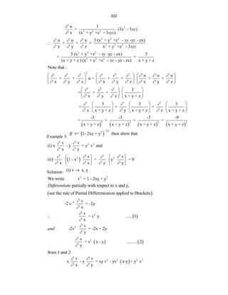
11.4 TOTAL DIFFERENTIATION
In Partial differentiation of a function of two or more variables , only one
variable varies. But in total differentiation, increments are given in all the
variables.
et z ( , )
L f x y

Let be the increment in z corresponding to the increments and in
z x y
  
x and y respectively
Replace by only


 
Then z ,
z f x x y y
  
   
 
, ( , )
z f x x y y f x y
  
    
     
, , , ( , )
z f x x y y f x y y f x y y f x y
    
        
     
, , , ( , )
r
f x x y y f x y y f x y y f x y
o z x
x y
   
 
 
     
   
  
   
   
y

Taking limits as 0, 0 we get
f f
x y z d x dy
x y
 
  
 
     
is called as total differential of z
d z
Let us see some Corollaries:
(1) Let
1 2 3
( , , ) and x= (t), y (t) ,z ( )
u f x y z t
  
  
[i.e. u is function of x,y,z and x,y,z each is a function of only one variable
t.]
Thus,
x,y,z t
u   

u u x u dz
t x t y t dt
u is a function of only one variable t,
d d dy u
d d d z
 
 

      

u u
We write total derivative and not
t t
d
d



 

2 2 2 2 3
. . If u= x + y + z , y=t , z= t
e g
then u x, y, z t
 

198. 198
        2
u
2x 1 + 2y 2t 2z 3t
t
d
d
  
(2) Let u= f(x, y) and (x, y) = 0

(x, y) = 0, y can be regarded as
a function of x and hence flow-diagram is

u x, y x
 
d u u u y
= 1 +
d x x y x
d
d
 
 
  
2 2
. . if u= x + y
e g
3 3 du
and x + y + 3xy = 4 then to find
dx
3 3
x + y + 3xy = 4
Differentiate with respect to x,
2 2 d y d y
3x + 3y + 3y + 3x = 0
d x d x
 
 
2
2
x + y
d y
=
d x x + y
 
2
2
d u u u d y x + y
= + = 2x +2y
d x x y d x x + y
and
 
 
 
 
 
 
   
   
2 2 2 2 2 2
2 2
2x x + y 2y x + y 2 x - y xy - x y
=
x + y x+y
 
 
 
 3)
 
d y
f x,y = 0 then to find
d x
If
 
result is a special case of result (4) .
This
   
u = f x, y and f x, y = 0
Let
u x, y
 
 
and f x, y = 0
y x
 
u x, y x
  
d u u u d y
then = +
d x x y d x
 
 

u
u = 0 = 0
x
d
d

u
y x
=
u
x
y
d
d




 
y f x
, =
x f y
d
or
d
 
 


199. 199
 
If u = f x, y, z
where y and z are all functions of x, then we have
u x, y, z x and
 
d u u u d y u d z
= + + ,
d x x y d x z d x
  
  
 
 
Also note that if f x, y, z = 0
u u d y u d z
then + + = 0
x y d x z d x
  
  
 
4)  
2
2
d y
f x, y = 0 then to find ,
d x
If
We use the following notations :
2 2 2
2 2
f f f f f
p = , q = , r = , s = , t =
x y x x y y
    
     
 
f x, y = 0
 
2
2
d y f x p
= - = - Result 5
d x f y q
 
 
 
  
 
2
2 2
d p d q
- p
d y d x d x
= - ..................(i)
d x q
q
 
 
  
 
 
p, q x, y x
 
d p p p d y
and = + =
d x x y d x
f f p
+
x x y x q
 
 
   
   
 
 
   
 
   
     
2 2
2
f f p p rq -sp
= - = r-s =
x x x q q q
 
  
 

 
 
dq q
dx y x y
q dy f f p
x dx y y q
    
     
    
    
     
    
2 2
2
f f p
x y y q
 
  
  
p
s t
q
 
sq pt
q



200. 200
2
2 2
d y 1 rp - sp sq - pt
from (i), = - q - p =
d x q q q
 
   
    
 
   
 
2 2
3
1
- q - 2pqs + p t
q
r
 
  
11.5 SOME ADDITIONAL RESULTS
Partial Diffferentiation applied to :
   
n 1 f
(1) Brackets : f (x, y, z) = n f (x, y, z)
x x
n
 
 

   
f
(2) Trignometric function : sin f (x, y, z) = cos f (x, y, z)
x x
 
 

   
f (x, y, z) f (x, y, z) f
(3) Expotential Function : a = a og a
x x
l
 
 
 
 
 
1 f
(4) Log - function : log f (x, y, z) =
x x, y, z x
f
 
 
 
 
(5) Inverse Trignometric function :
 
 
-1
2
1 f
sin f (x, y, z) =
x x
1- x, y, z
f
 
 

u 1
: (1) In general,
x
x
u
Note





. . if x = r cos and y = r sin
e g  
x
= cos
r
then



 
 
 
2 2 2
since , x + y = r
and
r
2r = 2x
x


r x
= = cos
x r




(i) and (ii),
from
x 1
r
r
x





(2) When we write
u x, y, z

It means u depeds on x, y, z and x,y,z are independent among themselves.
EXAMPLES

201. 201
TYPE – I
NOTE :
Problem in this type are based on direct differentiation
(1) First find dependent and independent variables.
(2) Use the necessary formulae.
Examples 1 :
y x
z = x + y then show that
If
2 2
z z
=
x y y x
 
    .
Solution:
y x
z = x + y z x, y
 
y-1 x
z
= yx + y log x .........(i)
y



y x-1
z
and = x log x + x y ..........(ii)
y


Differentiating (i) partially with respect to y,
 
2
y-1 y-1 x x-1
z 1
= y x log x + x y + log y xy
x y y

 
 
   
 
 
y-1 y-1 x-1 x-1
= y x log x + x + y + xy log y..........(iii)
 
Differentiating (i) partially with respect to x,
2
y y-1 x-1 x-1
z 1
= x + yx log x + 1 y + xy log y........(iv)
x y x

 
   
From (iii) and (iv)
2 2
z z
=
x y y x
 
   
Examples 2: 3 3 3
u = log (x + y +z 3 )
If xyz
 then show that
 
2
2
-9
+ + u =
x y z x + y + z
  
  
 
 
 
Solution:
Note that u is a function of x, y, z
i.e. u x, y, z

3 3 3
u = log (x + y +z 3 )
xyz

2
3 3 3
u 1
= (3x 3 )
x (x + y +z 3 )
yz
xyz


 

 
the rule of partial Differentiating applied to log function
see
similarly
and
2
3 3 3
u 1
= (3y 3 )
x (x + y +z 3 )
xz
xyz





202. 202
2
3 3 3
u 1
= (3z 3 )
x (x + y +z 3 )
xy
xyz




2 2 2
3 3 3
u u u 3 (x + y +z -y - zx)
+ + =
x y z x + y +z 3
xy z
xyz
  
  



2 2 2
2 2 2
3 (x + y +z -y - zx) 3
= =
(x + y + z ) (x + y +z - yz - zx) x + y + z
xy z
xy


Note that :
2
u u u
+ + u = + + + +
x y z x y z x y z
        
        
     
     
     
3
= + +
x y z x + y + z
  
  
   
   
   
3 3 3
= + +
x x + y + z y x + y + z z x + y + z
  
  
     
     
     
       
2 2 2 2
-3 -3 -3 -9
= + + =
x + y + z x + y + z x + y + z x + y + z
Example 3:
 
1 2
2
v= 1- 2xy + y then show that
If

 
2 3
2 2
v v
(i) x - y = y v and
x y
v v
(ii) 1 - x + y = 0
x x y y
 
 
   
   
 
 
   
   
Solution: (i) v x, y

2 2
We write v = 1 - 2xy + y
partially with respect to x and y,
Differentiate
 
see the rule of Partial Differentiation applied to Brackets .
-3 v
-2 v = -2y
x


 
3
v
= v y ...... 1
x



3 v
-2v = -2x + 2y
y
and


   
3
v
= v x - y .......... 2
y


from 1 and 2
 
3 3 2 3
v v
x - y = xy v - yv x-y = y v
x y
 
 

203. 203
   
2 2 3
v
(ii) 1 - x = 1 - x yv from (1)
x


   
2 2 3
v
1 - x = y 1 - x
x y x
v
  
  
 
 
    
 
 
y is constant, and v is a function of x, y
 
3 2 2 v
= y 2 + 1 - x 3v
x
xv


 

 
 
 
3 2 2 3
= y 2 + 3 1 - x v from (1)
xv y v
 

 
 
3 2 2
= yv 2 + 3 1 - x yv .........(3)
x
 

 
 
 
2 2 3
v
Again, y = y v x-y
y y y
  
  
 
 
 
   
2 2 3 3 2
v
= 3 v x x y - y + v (2xy -3y ) v x,y
y



   
2 3 2 3 3 2
= 3 v v x - y xy - y + v (2xy -3y )
 
  
 
   
3 2 2
= v y 3 v x - y xy - y + (2x -3y)
 
 
   
3 2 2
= v y 3 v x - y xy - y (2x -3y) ........(4)
 
 
 
2 2
v v
1 - x + y
x y y y
   
   
   
    
   
   
3 2 2 2 2
= y v -2x + 3y 1 - x v + 3 v y x- y + (2x -3y) from (3), (4),
 
 
   
3 2 2 2
=y v 3y 1 - x x- y v - 3y
 
 
 
3 2 2 2 2
= y v 3y 1 - x + x -2xy + y v - 3 y
 
 
3 -2 2
= y v 3y v v - 3y
 
 
 
 
2 2
= 0 v = 1 - 2 xy + y
Example 4 :  
u = log tan x + tan y + tan z then show that
If
u u u
sin 2x + sin 2y + sin 2z = 2
x y z
  
  
 
Solution: Here u x, y, z

 
Using the rule of partial diff. applied to log function we have,
2
u 1
= sec x
x tan x + tan y + tan z



2
u 1
= sec y
y tan x + tan y + tan z




204. 204
2
u 1
= sec z
x tan x + tan y + tan z



u u u
sin 2x + sin 2y + sin 2z
x y z
  
  
  
2 2 2
sin 2x . sec + sin2y . sec + sin2z. sec
=
tan + tany + tan z
x y z
x
 
 
2 tan x + tan y + tan z
= = 2
tan x + tan y + tan z
2
2
1
sin 2x. sec = 2 sin x . cos x . = 2 tan x
cos x
x
Examples 5 :
2 4t
n -r
= t , e then find the value of n show that
If 
2
2
1
r =
r r r t
    
  
 
 
 
Solution: We have r, t
 
 
To simplify the expression, we take log .
2
r
have, log = n log t -
rt
We 
Diff. partially with respect to r,
1 -2 r
=
r 4 t
 
 
r
= -
r 2
  


2
2 r
r = -
r 2 t
  


Diff. partially with respect to r,
2 2 3
2
1
r = - 3 r + r =
r r 2 r
1
- 3 r - ...... from (1)
2 t 2 t
r
r
    

  


   
    
   
 
 
 
2
2
2
1 1 r
r = - 3 - ........ (2)
r r r 2 2 t
   

 
 
 
    
   
Again diff. given relation with respect to t partially ,
2
2
1 n r 1
= +
t t 4 t
 
 

2
2
n r
= +
t t 4 t
 


 
  
 

205. 205
2
2
1
r = ,
r r r t
    
  
 
  
 
From (2) and (3) we get,
2 2
2 2
n 3 r 3
+ = - + n= -
4 t 2 t 4 t 2
r
t
   

Example 6 :  
-gx
u (x, t ) = A e sin n t - g x
If 
2
2
u u n
if = u hen show that g =
x x 2u
and t
 
 
Solution: u x, t

 
-gx
u
We have, = Ae cos n t - g x n
t


 
   
-gx
= An e cos n t - g x x is to be kept constant ........(1)
Again diff. u partially with respect to x, we get,
 
-gx -gx
u
= A -g e sin (nt - gx ) - g e . cos n t - g x
x


 
 
 
 
-gx
= -Ag e sin (nt - gx ) + cos n t - g x
 
 
 
Rule of partial differentitation applied to product
 
2
-gx
2
u
= -Ag -g e sin (nt - gx ) + cos n t - g x
x


 
  
 
-gx
e -g cos (nt - gx ) + g sin n t - g x

 
 
 
2 -gx
= + Ag e 2 cos (nt - gx )
2
2
u u
=
t x
 

 
From (1) and (2)

-gx 2 gx
(A n .e . cos (nt-gx) = . 2. Ag . e . cos (nt-gx)

2 n
n= 2 g g =
2



Example 7 :
2
2 -1 2 -1
y x u
u = x tan -y tan , then find .
x y x y
If

 
Solution: u x, y.

2 2 -1
2 2 2
2 2
u 1 1 1 x x
We have , = x - y -2y tan
y x
y x y y
1+ 1+
x y


 
 
  
 
 
   
3 2
-1
2 2 2 2
x
-2y tan
x xy
x y y x y
 
 
‟

206. 206
3 2
1
2 2
2 tan
x xy x
y
x y y


  

-1 x
= x - 2y tan
y
2
-1
u u x
= = 2 - 2y tan
x x y x y
y
   
    
   
   
   
2 2 2
2 2 2 2 2
2
1 1 2y x - y
= 1 - 2y = 1 - =
x y x + y x + y
1+
y
 
  
 
Check your progress:
2 2
1) If u, (x + y ) = x + y then show that :
u u u u
- = 4 1 - -
y x y
x
   
   
   
   
   
2 2
x + y u u
int u = u x, y find , .......
+ y y
H
x x
 
 
 
 
 
 
n 2
(2) Find the value of n so that u= r (3 cos - 1) satisfy the equation

2 u 1 u
+ in = 0
r sin
r s
r
  

    
   
   
   
u u
Hint : u r, , Find , ....... Ans. n = 2, -3.
r
 

  
 

 
 
xyz
(3) If u = e then show that
 
3
2 2 2 xyz
u
= 1+ 3xyz + x y z e
y z
x

  

2 3
u u
First find then
x z x y z
u
and
z
 
  
 

 
  
 
2
2
x
4a
(4) v = e , then prove that
t
c
If
t

2
2
2
v v
= a
t x
 
 
2
2
1
int : Take log, log v = log c - log - v x, t
2 4 t
x
H t
a
 
 
 
 
2
2
v v
(Find and , apply the rule of P.D. applied to log function)
t x
 
 
2
2 2 2
2 2 2 2
u 4
(5) Find where u = log (x + y + z ) Ans.
z (x + y + z )
yz
y

 

2 2
u u
(6) Verify =
y
x y
 
  
Where (i) u = log (y sin x + x sin y )

207. 207
m n
(7) If u = x y then show that
3 3
2
u u
=
z x
x y y
 
    
 
(8) u=log y sin x+ x sin x then show that
If
2 2
x y y y
u u
 
   

2 2 2
(9) If u=log x then show that
y z
 
 
2 2 2
2 2 2
2 2 2
x 1
x y z
u u u
y z
  
  
 
    
 
 
2u 2 2 2
int : e x u x,y,z
H y z
     

2u
2e 2x
x
u


 
-2u
u
e
x
x



 
2
-2u 2 -2u 2 -2e
2
u
e 2 e 2 e
x x
u e
u
x e xe x
 
 
 
     
-2u 2 -4u
= e 2 e
x

m 2 2 2
10) If u =r , r = x y z
 
2 2 2
2 2 2
then find the value of
x y z
u u u
  
  
 
 
2
2
2 2 2
2
Hint : u= x u x,y,z find , .......
x x
m u u
y z
 
 
 
   
 
 
  m
: m m+1 r
Ans
TYPE – II
Note :- Here we deal with the the problems of the type u = f (x, y, z )
where x, y functions of x, y, z
i.e. X, Y, Z x, y, z.
u  
We shall be frequently using the Chain- Rules can be develop drawing the
flow- diagram.
Example 8 :  
u u u
u=f x-y, y-z, z-x then show that + + =0
x y z
If
  
  
Solution: Let X=x-y, Y=y-z, Z=z-x
 
so that u=f X,Y,Z
u X,Y,Z x,y,z
 

208. 208
u u X u Y u Z
= + +
x X x Y x Z x
      
      
   
   
u u u u u
= 1 + 0 + -1=
X Y Z X Z
    
    
  
u u X u Y u Z
+
Y X y Y y Z y
and
      
      
    
     
u u u u
1 1 + 0
Y X Y Z
   
   
      
u u
=
Y X
 
 

u u X u Y u Z
Similarly +
Z X z Y z Z z
      
      
    
       
u u u u u
= 0 1 + 1 + ............. 3
X Y Z Y Z
    
    
      
(1), (2), (3)
From
u u u
+ 0
X Y Z
  
  
 
Example 9 :
2
x
u=f then prove that
y
If
 
 
 
2 2 2
2 2
2 2
u u u u u
(i) x + 2y =0 (ii) x + 3xy +2y =0
x y x x y y
    
     
 
 
 
Solution:
 
2
2
Let t= so that u=f t
x
y
2
x
that u is a function of only one variable =t, which in turn is a
Note
y




function of x and y
u t x,y ( see chain rule 2)
  
u u t u 2x
= =
x t x t y
d d
d d
 
 
  
2
2
u u t u -x
, = =
y t y t y
d d
and
d d
 
 
 
  
 
2 2
u u 2 u 2x u
x +2y 0
x y t y t
x d d
y d d
 
 
   
u u
. .x +2y 0.........................(1)
x y
i e
 
 

(1) partially with repect to y we get,
Diff

209. 209
2 2
2
u u u
x +1 2 0................(2)
x x x y
y
  
   
  
2 2
2
u u u
and x +2 y 2 0................(3)
x y y
x
  
   
  
 
Taking (2) x+ 3 y, we get
x

2 2 2 2
2 2
2 2
u u u u u u
x +2xy +xy +2y 2 0
x x y x x y y y
x y
     
       
 
  
 
 
u u
+2y =0 from (1)
y y
x
 
 
2 2 2
2 2
2 2
u u u
x +3xy 2y =0
x x y y
  
   
 
Example 10:    
dy
cos x sin then find
dx
y x
If y

Solution:
Taking logs, we get,
y log cos x = x log sin y
Let f (x,y) =y log cos x -xlog sin y=0
df dx
=-
df dy
dy
dx

 
f 1
Now, =y -sin x - log sin y
x cos x



= -y tan x-log sin y
f 1
and =log cos x- x cos y=log cos x-x cot y
y sin y


dy tan logsin
From (1)
dx logcos cot
y x y
x x y

 

Example 11:  
x y dy
y +x then find
dx
x y
If x y

 
Solution:
   
Let f x+y
x y x y
x y y x o

    
dy f x
..................(1)
dx f y
 
 
  
  
 
x+y x y-1
f
, = x+y 1+log (x+y) -y logy-y x
x
Now


 
  
 
x+y x-1 y
f
and = x+y 1+log (x+y) -xy x logx
y




210. 210
  
 
 
  
 
 
x+y x y-1
x+y x-1 y
x+y 1+log (x+y) -y logy-yx
y
From (1), =
x x+y 1+log (x+y) -xy - x logx
d
d



Example 12: Pr that at a point of the surface
ove x y z
x y z =c
 
2
1
where x=y=z, log
y
z
x ex
x

 

 
Solution:
2
From the expression it is clear that z x,y
x y
z

 
 

 
 
logs
Taking
x log x+y log y+z log z =log c
Different with respect to y partially, (i.e. keeping x constant)
1 1 z
0+log y+y log z+z
y z y


 
  
 
 
 
 
2
1 log
z
x 1 log
y
z



 

. with respect to x partially, we get,
Diff
 
 
2
2
z 1 1 z
1 log
x y x
1 log
y
z
z
 
  
 

   
 

 
 
 
 
2
1 log z
=
x
1 log
y
z z




 
 
1 log
z
, can show (as in (1) that
x 1 log
x
Now we
z



 

  
 
2
1 log 1 log
z
From (2),
x y 1 log
x y
d d z z
  
  

 
   
2
2
3
1 log
z 1
x=y=z,
x y 1+log x
1 log
x
At
d d x
x x
 
   

   
1 1
= =
log e+log x log e x
x x
 
 
1
= log ex
x

  
 
Check your progress:
 
(1) z=f x,y,u,v where u,v are functions of x,y then prove that
If

211. 211
z f f u f v
= + + and write corresponding formulae for
x x u x v x
     
     
 
z
y


.
z
Hint : z x,y,u,v , =.............
x
x y


 
 
 
 
 
2 2 2
(2) If v=f x then show that
y z
 
     
2 2 2
2 2 2 2 2 2 2 2 2
2 2 2
f v v
4 x f ' x 6 x
x y z
y z y z f y z
  
  
         
2 2 2
int : Let x
H y z u
   

v u x,y,z
  
v u u
and proceed
x v x
  
  

   

11.6 TYPE - III VARIABLE TO BE TREATED AS
CONSTANT
Notations :
u
x


 
 
 
means partial derivative of u with respect to x keeping
Y constant.
To find
u
x y


 
 
 
we must have an equation in u, x and y only.
Example 13: x=r cos , y=r sin then show that
If  
2
2 2
x y
x ,
r r
Where surffixes denote variables kept constant
y x y
 
 
 
 
   
  
   
 
   
 
Solution:
x=r cos , y=r sin
 
y
cos , sin .
r
x
r

 

 
   
 
   
 
   
 
2
2
2 2 2
x y
x x cos y sin r cos r sin
r r
y
 
 
   
 
 
   
 
     
   
   
   
 
2 2 2
r = x +y

Example 14: If u= x+my, v=mx- y, then show that:
l l

212. 212
2
2 2
u x
(i) and
x u
y v m
  
  
   
 
   

   
2
2 2
y v
(ii)
v y
x u
m
  
  
 
 

 
 

   
Solution: We have
u= x+my
l
v=mx- y
l
(i) u= x+my
l
u
....................(1)
x y
l


 
 
 
 
v
x
( ) To find we must have relation between x,u and v
u
ii


 
 
 
Eliminating y from the given relations, we get,
 
2 2
u+mv= x
l l m

2 2
x=
lu mv
l m


2 2
v
x 1
............(2)
u l m


 

 

 
(1) and (2)
From
2
2 2
y v
u x
x u
l
l m
 
 
   
 
   

   
( ) v= mx- y ..............(3)
iii l
Diff with respect to v keeping x constant,

x
y
=0-
v
l l


 
 
 
x
y 1
y l


 
 
 
 
u
v
(iv) To find , lim x from given relations,
y
we e inate


 
 
 
 
2 2
i.e. mu-lv l m y
 
 
2 2
u
v
0- = 1
y
l l m


 
  
 
 
2 2
u
v
=-
y
l m
l


  
  
 
From (4), (5)


213. 213
2 2
2
x u
y v
=
v y
l m
l
 
 
  
 
 
 
   
Example 15:  
f x,y,z 0 then show that
If 
z 1
x
x
z
y
y




 

 
 
 
 
 
Solution:
 
Here we use the result that if f x,y 0

f
y x
f
x
y
y
then

 



 
 
(i) Here f x,y,z =0. When y is kept constant,
y
z f x
We have, =-
x f z
  
  
 
 
 
y
x f z
( ) And =-
z f x
ii
  
  
 
 
 
z 1
From (1) and (2)
x
x
z
y
y




 
 
 
 
 
 
 
Example 16:
cos sin
x= , y= , evaluate
u
If
u
 
x u u u
u x x y
y x
 
   
   
 
     
   
     
       
Solution
cos
(i) x=
u

2
x cos
= - ................(1)
u u

 

 
  
 
2
2
sin
( ) y = -
u
ii


2
y sin
= .....................(2)
u u

 

 
  
 
u
(iii) To find , we eliminate from given relations,
u 



 
 
 

214. 214
2 2
2
1
i.e. x y
u
 
2
2 2
1
u ............................( )
x
or A
y


 
2
2 2
u 2
2u
x x
y
x
y



 
 
 
  
 
2
2 2
u
...................(3)
x u x
y
x
y



 
 
 
  
2
2 2
1
(iv) and again
x
u
y


 
2
2 2
u 2
2u
y x
x
y
y


  
 
 
  
 
2
2 2
u
......................(4)
y u x
y
y
y


  
 
 
  
(1), (2), (3), (4) we get,
From
   
2 2
2 2
2 2 2 2
cos sin
Required expression = -
u u
u x u x
x y
y y
 
   
 
   
   

   
   
   
 
   
 
2
3 2 2
cos + y sin
=
u x
x
y
 

2 2
cos sin 1
but x cos sin
u
y
u
 
 

  
 
2
4 2 2
1
Re expression =
u x
quired
y

4
4
1
= u 1 (from A)
u
 
Example 17: 2 2 2 2 2 2
x+y+z+u+v=a, x +y +z +u +v =b ,
If
where a,b are constants, prove that
y,z , ,
,
u x v y
x u y v
v z u z
x z
   
   
 
     
  
 
     
     
 

215. 215
Solution:
y,z
u
To find to eliminate v from the given equations and as this
x
we have


 
 
 
process will have to be repeated four times, we proceed in the following way.
Let x+y+z+u+v=a ..................(1)
2 2 2 2 2 2
x +y +z +u +v =b ..............(2)
differentiating with respect to x partially keeping y,z as constants, we get,
y,z ,
u v
1+ 0 .........(3)
x x y z
 
 
   
 
   
   
y,z ,
u v
and 2x+2u 2y 0 ..........(4)
x x y z
 
 
   
 
   
   
y,z
u
Solving the equations (3), (4) for by Cramer's Rule we get
x


 
 
 
y,z
u v-x
..........(5)
x u-v


 

 
 
differentiating (1), (2) partially with respect to y keeping x, z as
Similarly
constants, we have
x,z , x,z
u v v
1+ 2 0..............(7)
y y y
x z
v
  
  
     
  
     
     
x,z ,
u v
ey+ex 2v 0
y y x z
 
 
   
 
   
   
x,z
v
(6), (7) for we get
y
Solving


 
 
 
x,z
v y-u
.........(8)
y u-v


 

 
 
Similarly differentiating (1), (2) partially with respect to u treating v,z as constant
we get,
u,z ,
x u
1 0 ............(9)
u u v z
 
 
   
  
   
   
v,z ,
x y
and 2x 2y 2 0 .............(10)
u u v z
u
 
 
   
  
   
   
v,z
x
solving (9), (10) for e get,
u
w


 
 
 
v,z
x
....................(11)
u
y u
x y



 

 

 

216. 216
Similarly differentiating (1), (2) partially with respect to v where u,z, are kept
constants, we get,
, ,
1 0 ..... (12)
u z u z
x y
v v
 
   
  
   
 
   
, ,
2 2 2 0.........(13)
u z u z
x y
x y v
v v
 
   
  
   
 
   
,
equations (12), (13) for we get,
u z
y
Solving
v

 
 

 
,
-
....................(14)
-
u z
y v x
v x y

 

 

 
From (5), (11) and from (8), (14) we get,
, , ,
,
- -
- -
y z v z u z
x z
u x v x y u v y
x u u v x y y v
 
   
     
    
 
     
   
     
 
Example 18: 2 2
If and
u x y
  3 ,
x s t
 
2
2
2 - . Find .
u
y s t
t



2 2
Solution: We have u x y
 
2 , 2
u u
x y
x y
 
  
 
Now, , ,
u x y s t
 
u u x u y
s x s y s
    
    
    
(2 ) (1) (2 ) (2)
x y
 
2 4
x y
 
2
2
Now, (2 4 )
u u
x y
s s s s
   
 
  
 
   
 
x y
=2 + 4
s s
 
 
=2 1+4 2=10
 
u u x u y
And = + .............(i)
t x t y t
    
    
 
= 2x 3 +2y (-1)

= 6x-2y
2
2
u u
And = = (6 2 )
t t t t
x y
   
   
 

 
 
2
x y
= 6 -
t t
x
 
 

217. 217
= 6(3)-2(-1)=20 ......................(ii)
Check Your Progress-
y y
(1) x=r cos , y= r sin then show that 1
r r
If
 
 
 
 
   

   
   
 
z x y
(2) If x,y,z 0 then show that 1
y z x
y z
x
  

  
     
    
     
   
 
(3) If u=ax+by, v=bx-ay, show that
u x y v
1
x u v y
y v x u
   
   
 
     
   
 
     
       
11.7 LET US SUM UP
In this chapter we have learn Application of Differential equation like-
Partial Derivative of 1st order and 2nd order
Total differentiation
Euler's Theorem
Approximation and error formula
Maxima and Minima of the function.
11.8 UNIT END EXERCISE
cos
1. and if .cos( sin ).
r
u u
Find u e r
r



 

 
1 1
2. +y if sin tan .
u u x y
Find x u
x y y x
 
 
   
   
 
   
 
1
2 2 3
2
3. If (1 2 ) then prove that .
u u
u xy y x y y u
x y
  
    
 
1
2 2 2
2
4. If (1 2 ) then prove that (1 ) 0.
u u
u xy y x y
x x y y
  
   
 
     
   
   
   
2 2 2
2 1 2 1
2 2
5. If tan tan then prove that .
y x u x y
u x y
x y y x x y
     
 
  
     
  
 
2
3 3 3
2
9
6. If log( +z ), then prove that .
( )
u x y xyz u
x y z x y z
 
  
     
 
    
 

218. 218
3 3
1
2 2 2
2 2
2 2
7. If tan , then show that
(i) sin2 .
(ii) 2 2cos3 sin .
x y
u
x y
u u
x y u
x y
u u u
x xy y u u
x y
x y
  

  
 

 
 
 
 
  
  
 
 
4 4
8. If log , then show that 3.
x y u u
u x y
x y x y
 
  
  
 
 
  
 
*****

219. 219
MEAN VALUE THEOREMS 12
Unit Structure
12.0 Objectives
12.1 Introduction
12.1.1 Rolle‟s Theorem:
12.1.2 Lagrange‟s Mean Value Theorem
12.1.3 Another Form of Lagrange‟s Mean Value Theorem:
12.1.4 Geometrical Interpretation of Lagrange‟s Mean Value Theorem:
12.1.5 Some Important Deductions from the Mean Value Theorem:
12.2 Cauchy‟s Mean Value Theorem:
12.2.1 Another Form of Cauchy‟s Mean Value Theorem:
12.2.2 Geometrical Application of Cauchy‟s Mean Value Theorem
12.3 Summary
12.4 Unit End Exercise
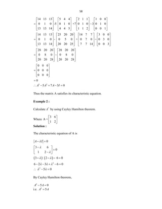
12.0 OBJECTIVES:
After going through this chapter you will be able to:
 State and prove three mean value theorems (MVT): Rolle‟s MVT,
Lagrange‟s MVT and Cauchy‟s MVT.
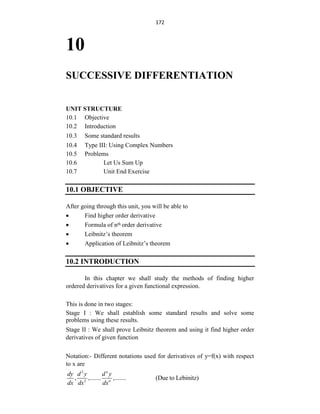
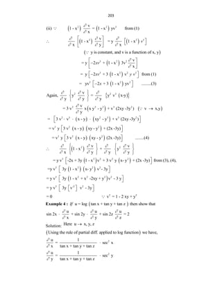
12.1 INTRODUCTION:
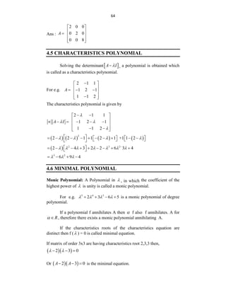
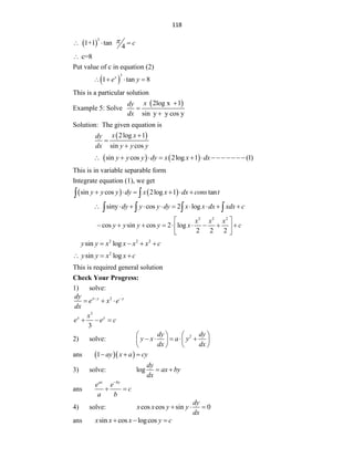
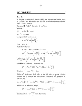
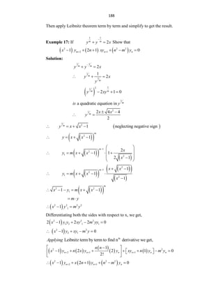
The Mean Value Theorem is one of the most important theoretical tools in
Calculus. Let us consider the following real life event to understand the concept
of this theorem: If a train travels 120 km in one hour, then its average speed
during is 120 km/hr. The car definitely either has to go at a constant speed of 120
km/hr during that whole journey, or, if it goes slower
(at a speed less than 120 km/hr) at a moment, it has to
go faster (at a speed more than 120 km/hr) at another
moment, in order to end up with an average speed of
120 km/hr. Thus, the Mean Value Theorem tells us
that at some point during the journey, the train must
have been traveling at exactly 120 km/hr. This
theorem form one of the most important results in
Calculus. Geometrically we can say that MVT states
that given a continuous and differentiable curve in an
interval [a, b], there exists a point c ∈ [a, b] such that
the tangent at c is parallel to the secant joining (a, f(a)) and (b, f(b)).
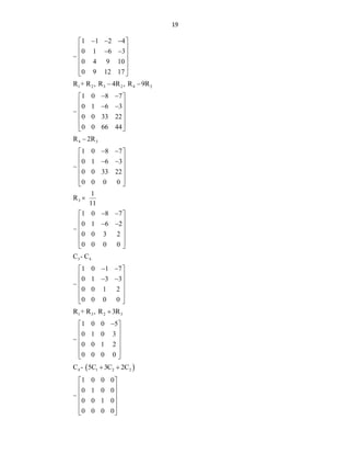
12.1.1 Rolle’s Theorem:
If f is a real valued function such that (i) f is continuous on [a, b], (ii) f is
differentiable in (a, b) and (iii)f(a) = f(b) then there exists a point c  (a, b) such
that  
f c 0
 

220. 220
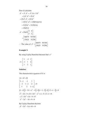
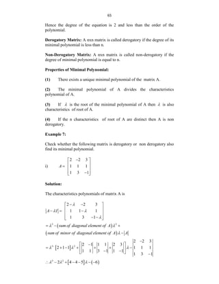
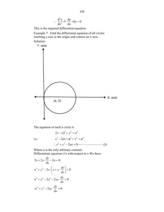
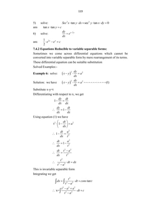
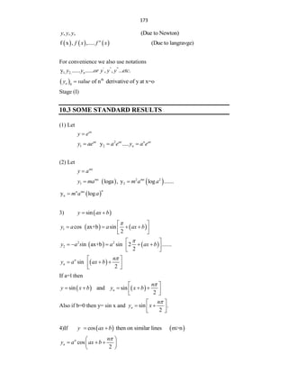
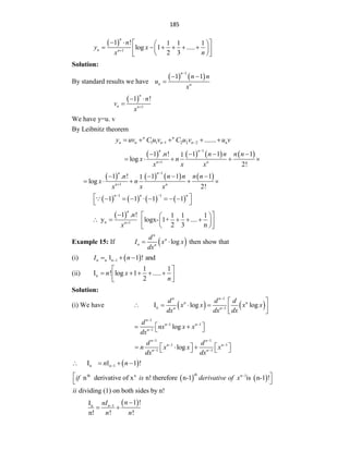
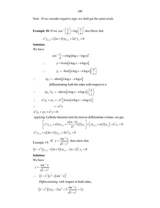
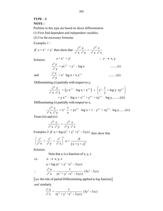
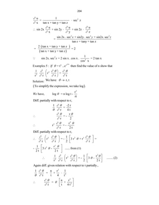
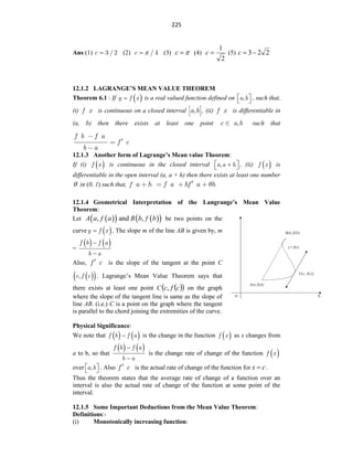
Geometrical Interpretation of Rolle’s theorem:
Fig 12.1
We know that f c
( )
 is the slope of the tangent to the graph of f at x = c. Thus the
theorem simply states that between two end points with equal ordinates on the
graph of f, there exists at least one point where the tangent is parallel to the X
axis, as shown in the
Fig 12.1. After the geometrical interpretation, we now give you the algebraic
interpretation of the theorem.
Algebraic Interpretation of Rolle's Theorem:
We have seen that the third condition of the hypothesis of Rolle's theorem is that
f(a) = f(b). If for a function f, both f(a) and f(b) are zero that is a and b are the
roots of the equation f(x) = 0, then by the theorem there is a point c of (a, b),
where f c
( )
 = 0, which means that c is a root of the equation f x
( )
 = 0.
Thus Rolle's theorem implies that between two roots a and b of f(x) = 0 there
always exists at least one root c of f x
( )
 = 0 where a < c < b. This is the
algebraic interpretation of the theorem.
Example 1: Verify Rolle‟s Theorem for the following:
(1)
2
x in [ 1,1]
 (2)
2
x in 1,3
 
 
Solution: (1) Let   2
x
x
f  , x [ 1,1]

As  
x
f is a polynomial in x, it is continuous and differentiable everywhere on
its domain. Also     1
1
1 

 f
f
 The conditions of the Rolle‟s theorem are satisfied.
 We may have to find some c [ 1,1]
 such that  
f c 0
 
Now   2
x
x
f   
f x x
2 .

   
f c c
2 .

 
 
f c c
0 2 0

    c 0
  and lies in [ 1,1]

 Rolle‟s Theorem is verified.
2) Let  
f x x2
,
 x 1,3
 
  
 
x
f is polynomial in x.  f(x) is continuous and differentiable everywhere on
its domain. i.e. (i) f is continuous on [1, 3] and (ii) f is differentiable in (1, 3).
But we have  
f 1 1
 and  
3
f 9 which are not equal.
 The values of f at the end points are not equal i.e.    
f f
1 3

 The function
2
x in (1, 3) do not satisfy all the conditions of Rolle‟s Theorem.

221. 221
Example 2: Verify Rolle‟s Theorem for     x
f x x x e /2
3 
  in 3,0
 

 
Solution: Given     x
f x x x e /2
3 
  in 3,0
 

 
(i)  
f x is continuous in 3,0
 

  since it is a product of continuous functions.
(ii)      
x x
f x x e x x e
/2 2 /2
1
2 3 3
2
 
 
     
 
 
= x x x
e x
2
/2 3
2 3
2 2

 
  
 
 
 
= x x x
e
2
/2
3
2 2

 
  
 
 
 
exists in (-3, 0)
(iii)    
f f
3 0 0.
   
All conditions of Rolle‟s Theorem are satisfied.  There exists  
c 3,0
  such
that  
f c 0
  c c c
e
2
/2
3 0
2 2

 
    
 
 
 
c c
2
6 0 c c
2
6
   = 0
c = 3, -2
c c
3 3,0 3, 2 3,0
Hence Rolle‟s theorem is verified and c = - 2 is the required value.
Example 3: Verify Rolle‟s Theorem for  
f x =
 
x ab
x a b
2
log
 

 
 

 
in a b
,
 
  ;
a, b > 0
Solution:  
x
f is continuous in (a, b) and  
f x =
   
x ab x a b
2
log log log
   
 
 
x x ab
f x
x
x ab x x ab
2
2 2
2 1 

   
 
exists, since it is not indeterminate or
infinite.
Also    
f a f b 0
   All conditions of Rolle‟s Theorem are satisfied.
 There exists  
c a b
,
 such that  
f c 0
 

 
c ab
c c ab
2
2
0



(i.e.) c ab
2
0
  c ab
  , which lies in (a, b).
Example 4: Verify Rolle‟s Theorem for  
f x =  
x
e x x
sin cos

 in
[ / 4,5 / 4].
Solution: Since
x
e
, sinx, cosx are continuous and differentiable functions, the
given functions is also continuous in
5
,
4 4
 
 
 
 
and differentiable in
5
,
4 4
 
 
 
 
Also,    
f e /4
/ 4 sin / 4 cos / 4 0

  

  

222. 222
   
f e 5 /4
5 / 4 sin5 / 4 cos5 / 4 0

  

  
 
f / 4

 =  
f 5 / 4
 = 0
Hence, Rolle‟s Theorem is applicable.
Now,      
x x
f x e x x e x x
sin cos cos sin
 
      = x
e x
2 cos

  c
f c e c
'
2 cos 0

  2
/


c , which lies in
5
,
4 4
 
 
 
 
Example 5: Verify Rolle‟s theorem for f(x) = x
2
sin , x
0 
  .
Solution: We have f(x) = x
2
sin , x
0 
 
Since x
sin is continuous and differentiable on [0,  ], x
2
sin is also continuous
and differentiable in the given domain. Now  
f 0 =  
f  = 0
all the conditions of Rolle‟s Theorem are satisfied.
 The derivative of  
x
f should vanish for at least one point  
c 0,
 such
that  
f c
'
0
 Now, f x x x x
2sin cos sin2 .
 
f c c
'
sin2 .
  ⇒  
f c c
'
0 sin2 0
   ⇒ c
2 0, , ,.
2 .
,3 .
c 0, ,
2
,...


 
Since c =
2

lies in  
0, , it is the required value. Hence Rolle‟s theorem is
verified.
Example 6: If  
f x ,  
x
 ,  
x
 are differentiable in a b
( , ) , show that there
exists a value c in (a, b) such that
f a a a
f b b b
f c c c
( ) ( ) ( )
( ) ( ) ( )
( ) ( ) ( )
= 0
Solution: Consider the function  
F x defined by, F(x) =
( ) ( ) ( )
( ) ( ) ( )
( ) ( ) ( )
f a a a
f b b b
f x x x
Since  
x
f ,  
x
 ,  
x
 are differentiable in a b
( , ),  
F x is also differentiable in
 
b
a, . Further,  
F a 0
 and  
F b 0
 since in each case, two rows of the
above determinant becomes identical.    
F a F b
 
Hence by Rolle‟s Theorem, there is a value  
b
a
c ,
 such that F c 0
i.e
f a a a
f b b b
f c c c
( ) ( ) ( )
( ) ( ) ( )
( ) ( ) ( )
= 0
Example 7: If  
f x =    
x x x x
1 2 3
   then show that  
f x has
three real roots in [– 3, 0].

223. 223
Solution: We apply Rolle‟s Theorem to  
f x in three intervals 1,0
 

  ,
2, 1
 
 
  , 3, 2
 
 
 
We observe that
(i)  
f x is continuous in all the intervals since it is a polynomial in x.
(ii)  
f x is differentiable in all the intervals  polynomial in x.
(iii)      
f f f f
3 2 1 (0) 0.
      
Hence Rolle‟s Theorem is applicable in all each interval such that  
f c 0
 
 
f x
 has three real roots.
Example 8: Prove that between any two real roots of the equation,
x
e x
sin 1
 there is at least one roots of x
e x
cos 1 0
  .
Solution: Let a and b be two real roots of the equation x
e x
sin 1

(i.e.) of
x
e
x 

sin (i.e.) of x
e x
sin 0
 
Let   x
f x e x
sin

  , which is continuous and differentiable.
Also,    
f a f b 0
  . Since a and b are roots of  
f x .
 By Rolle‟s Theorem there is at least one real value c between a and b such
that  
f c
'
0

Now,  
f x
 = x
e x
cos

 
  c
f c e c
cos


   
  c
f c e c
'
0 cos 0

    
c
c
e c
e c
cos 0
cos 1 0

 
  
 c is a root of x
e x
cos 1 0
  lying between a and b.
Example 9: Us Rolle‟s Theorem to prove that the equation
a b
ax bx
2
3 2
  
has a root between 0 and 1.
Solution: Let  
x
f =
ax bx a b
x
3 2
3 2 3 2
 
  
 
 
which is obtained by integrating
the given equation.
Here  
f x is continuous in 0,1
 
  and differentiable in (0, 1) and
   
f f
0 1 0
 
By Rolle‟s Theorem there is a value  
c 0,1
 such that  
f c 0
 
Now,   a b
f x ax bx
2
3 2
 
    
 
 
and this is zero at x = c which means the
equation,
a b
ax bx
2
3 2
 
  
 
 
has a root between 0 and 1.

224. 224
Example 10: Show that the equation x x
3
1 0
   where x  has exactly
one real root.
Solution: Let  
f x x x
3
1,
   x 
 
f 0 1 0
   and  
f 1 1 0
 
Since  
f x is a polynomial, it is continuous.
Thus, using Intermediate value theorem, we get, there is a number c between 0
and 1 such that  
f c 0

Thus the given equation has a root.
Now, let if possible  
f x have two roots, say a and b. Then  
f a =  
f b 0
 .
Since  
f x represents a polynomial, it is differentiable on (a, b) and continuous
on a b
,
 
 
Thus by Rolle‟s Theorem there exists a member c between a and b such that
 
f c 0
 
But  
f x x2
3 1,
   x 
 
f x 1

  , x
 
Hence  
f x 0
  for any x, which is a contradiction.
Thus, the equation  
f x = 0 cannot have two real roots.
 The equation x x
3
1 0,
   x  has exactly one root.
Check Your Progress
1. Verify the validity of the conditions and the conclusion of Rolle‟s
Theorem for the function f defined on the intervals as given below:
a) x x
2
3 2
  on 1,2
 
 
b)
x
x
2
6
log
5
 

 
 
 
on 2,3
 
 
c) x
e x
sin

on [0, ]

d)  
x
e x x
sin cos
 on / 4,5 / 4
 
 
 
e)  
x x
2 2
1  on 0,1
 
 
f)    x
x x e
1 3 
  in 1,3
 
 
2. Prove that the equation x x x
3 2
2 3 1 0
    has at least one root
between 1 and 2.
3. Test whether Rolle‟s Theorem holds true for  
x
f = x in  
1
,
1

4. Verify Roll‟s Theorem for the function  
x
f = x
e
x
sin
in  

,
0
5. Show that 0
1
4
3


 x
x has exactly one real solution.

225. 225
Ans:(1) c 3 / 2
 (2) c / 4

 (3) 

c (4)
2
1

c (5) 2
2
3

c
12.1.2 LAGRANGE’S MEAN VALUE THEOREM
Theorem 6.1 : If  
y f x
 is a real valued function defined on a b
,
 
  , such that,
(i) f x is continuous on a closed interval ,
a b , (ii) f x is differentiable in
(a, b) then there exists at least one point ,
c a b such that
f b f a
f c
b a
12.1.3 Another form of Lagrange’s Mean value Theorem:
If (i)  
f x is continuous in the closed interval a a h
,
 

  , (ii)  
f x is
differentiable in the open interval (a, a + h) then there exists at least one number
 in (0, 1) such that, f a h f a hf a h
12.1.4 Geometrical Interpretation of the Langrange’s Mean Value
Theorem:
Let  
   
 
, and ,
A a f a B b f b be two points on the
curve  
y f x
 . The slope m of the line AB is given by, m
=
   
f b f a
b a


Also, f c is the slope of the tangent at the point C
 
 
c f c
, . Lagrange‟s Mean Value Theorem says that
there exists at least one point C  
 
c
f
c, on the graph
where the slope of the tangent line is same as the slope of
line AB. (i.e.) C is a point on the graph where the tangent
is parallel to the chord joining the extremities of the curve.
Physical Significance:
We note that    
f b f a
 is the change in the function  
f x as x changes from
a to b, so that
   
f b f a
b a


is the change rate of change of the function  
f x
over a b
,
 
  . Also f c is the actual rate of change of the function for c
x  .
Thus the theorem states that the average rate of change of a function over an
interval is also the actual rate of change of the function at some point of the
interval.
12.1.5 Some Important Deductions from the Mean Value Theorem:
Definitions:-
(i) Monotonically increasing function:

226. 226
Let  
f x be defined in a b
,
 
  . Let 1 2
, ,
x x a b such that 1 2
x x . If
1 2
f x f x then  
f x is said to be a monotonically increasing function.
(ii) Monotonically decreasing function:
Let  
f x be defined in a b
,
 
  . Let 1 2
, ,
x x a b such that 1 2
x x . If
f x f x
1 2
then  
f x is said to be a monotonically decreasing function.
Note:
(i) If  
f x is monotonically increasing  
 in a b
,
 
  then we can write
     
f a f x f b
  for all  
x a b
,
 .  
f a is its minimum value and  
f b is
its maximum value.
(ii) If  
f x is monotonically decreasing  
 function in a b
,
 
  then we can
write,      
f a f x f b
  for all  
x a b
,
 .  
f a is its maximum value and
 
f b is its minimum value.
(iii) Let  
f x be differentiable in an interval (a, b). Let  
x x a b
1 2
, ,
 and
2
1 x
x  then applying Lagrange‟s Mean Value Theorem to x x
1 2
,
 
  , we get
2 1
2 1
f x f x
f c
x x
or 2 1 2 1
f x f x x x f c (*)
(1) Let 0
f x for every value of x in  
a b
, then from equation (*)
   
f x f x
2 1
0
  for  
x x
2 1
 and  
f c
 both are positive i.e.
   
f x f x
2 1

We have thus proved: A function whose derivative is positive for every value of
x in an interval is a monotonically increasing function of x in that interval.
(2) Let 0
f x for every value of x in (a, b) from equation we have,
   
f x f x
2 1
0
     
f x f x
2 1
 
for x x
2 1
 is positive and f c negative.
Hence  
f x is a decreasing function of x.
We have thus proved: A function whose derivative is negative for every value of
x in an interval is a monotonically decreasing function to x in that interval.
Example 11: Verify mean value theorem for log
f x x on e
1,
 
 
Solution: The given function is log
f x x on e
1,
 
 
We know that log
f x x is continuous on e
1,
 
  and differentiable on (1, e).
Thus all the conditions of Lagrange‟s mean value theorem are satisfied.
  
c e
1,
  such that
   
 
f e f
f c
e
1
1





227. 227
 
e
f c
e
log log1
1


 

Since loge = 1, log1 = 0 and
1
f x
x
we get
e c
1 1
1


c e 1
   which lies in the interval (1, 2) and hence in (1, e), since 2 < e < 3.
Example 12: Separate the interval in which the polynomial
x x x
3 2
2 15 36 10 is increasing or decreasing.
Solution: We have,  
f x = x x x
3 2
2 15 36 10
2
6 30 36
f x x x
(i)  
f x is an increasing function if 0
f x
i.e. 2
6 30 36 0.
x x i.e. 2
5 6 0
x x
But x x x x
2
5 6 ( 3)( 2)
    
x x
2
5 6 0
    if ( 3 0
x and x 2 0) or (x 3 0 and
x 2 0)
i.e. if (x 3
 and x 2
 ) or (x 3
 and x 2
 )
i.e. if x 3
 or x < 2
Hence  
f x is an increasing function if x lies in  
,2
 or  
3,
(ii)  
f x is a decreasing function if 0.
f x
i.e. x x
2
6 30 36 0
  
i.e.if x x
2
5 6 0
  
But x x x x
2
5 6 ( 3)( 2)
    
x x
2
5 6 0
    if (x 3 0
  and x 2 0
  ) or (x 3 0
  and x 2 0
  )
i.e. if (x 3
 and x 2
 ) or (x 3
 and x 2
 )
i.e. if x 3
 and x 2
 since x 3
 and x 2
 is impossible.
i.e. if x
2 3
  ⇒  
f x is decreasing in (2, 3)
Thus  
f x is increasing in  
,2
 and  
3, and  
f x is decreasing in (2, 3).
Example 13: Find the interval in which
1
f x x
x
is increasing or
decreasing.
Solution: We have
1
f x x
x 2
1
1
f x
x
2
2
1
x
f x
x
(i)  
f x is an increasing function if 0
f x
i.e. if .
0
1
2
2


x
x
i.e. if .
0
1
2


x
i.e. if 1
2

x ⇒ 1

x or 1


x

228. 228
Hence  
f x is increasing in the interval  
,1
 and  
1,
(ii)  
f x is a decreasing function if 0.
f x
i.e.
2
2
1
0
x
x
2
1 0
x i.e if x 2
< 1.
i.e. if 1

x ⇒ 1
1 

 x
Hence  
f x is decreasing in (-1, 1).
Example 14: Show that if ,
0

x
2 2
log 1
2 2 1
x x
x x x
x
for
.
0

x
Solution: Let us assume,
2
log 1
2
x
f x x x
  x
f x x
x x
2
1
1 .
1 1

    
 
 
f x 0

  for all 0

x except at x 0.
 and f(0) 0.

 
f x
 is an increasing function in  
0,
 
f x
 increasing from 0 and hence  
f x 0
 .
x
x x
2
log(1 )
2
   , for x 0

… (i)
Consider,
 
 
 
x
f x x x
x
2
log 1
2 1
   

 
   
x x x
f x
x
x x
2 2
'
2 2
2 1
1
1
2 1 2 1

   

 
 
f x 0

  for x 0
 except at x 0
 when it is zero.
 
f x is an increasing function in  
0,
 
f x increasing from 0 and hence  
f x 0.

 
 
x
x x
x
2
2
log 1
2 1
   

for x 0.

… (ii)
From (i) and (ii),  
 
x x
x x x
x
2 2
2
log 1
2 2 1
    

for x 0.


229. 229
Example 15: Show that x y x y
1 1
tan tan
 
  
Solution: Let    
f x x
1
tan

 By Lagrange‟s Theorem,
     
c
f
a
b
a
f
b
f '



   
x y
x y c
1 1
2
tan tan 1
1
 

 
 
for x c y
2 2
 
    
But,
c2
1
1
1


( 2
c
 is positive)
x y
x y
1 1
tan tan
1
 

 

x y x y
1 1
tan tan
 
   
Example 16: Show that  
x e
x
x
10
10
log
log 1
1 
 

where x 0
 and
1
0 

Solution: Let  
f x =  
x
10
log 1

 By second form of Lagrange‟s MVT
For x
0,
 
  we have,
f a h f a hf a h
putting, a = 0 and h = x.
     
f x f xf x
0 

 
=    
xf x xf x
0  
 
 
But,  
  e
f x
x
1
1 log 10
 

 
  e
e
f x
x
x
10
log
1
1
1 log 10




  


But, f x xf x
 
 
f x e
f x
x x
' 10
log
1


  

 
x e
x
x
10
log
log 1
1 
  

Example 17: Applying Lagrange‟s M.V.T. to
x
e , determine  in terms of a
and h. Hence deduce that,
x
e x
x x
1
0 log 1.
 

 
 
 
 
Solution: Let   x
f x e
   x
f x e

 

230. 230
Now,      
f a h f a hf a h
'

   
 
a h
a h a
e e he



  
 
a h a h
e e he e
1 . 
  
h
h e
e
h
1
 

h
e
h
h
1
log

 

 
 
 
 
h
e
h h
1 1
log

 

 
 
 
 
But, 0 1

 
h
e
h h
1 1
0 log 1
 

 
  
 
 
Now by substituting h = x in the above equation, we get,
x
e
x x
1 1
0 log 1
 

 
  
 
 
Example 18: Show that,    
b a b a
b a
b a
1 1
2 2
tan tan
1 1
 
 
  
 
Hence show that 1
3 4 1
tan
4
4 25 3 6
 
  
   
 
 
Solution: Let    
f x x
1
tan
 in a b
,
 
 
 
f x
x2
1
1

 

 By Lagrange‟s M. V. T.
 
   
f b f a
f c
b a

 

where  
c a b
,

   
b a
b a
c
1 1
2
tan tan
1
1
 

 


(1)
Since a c b,
  a c b
2 2 2
 
a c b
2 2 2
1 1 1
     
a c b
2 2 2
1 1 1
1 1 1
  
  
(2)
From (1) and (2)
b a
b a
b a
1 1
2 2
1 tan tan 1
1 1
 

 

 
2
1
1
2
1
tan
tan
1 a
a
b
a
b
b
a
b







 

(3)
For the second part;
Since 1
tan
4


 we put a = 1 and b
4
3
 in (3)

231. 231
 
   
1 1
4 4
1 1
3 3
4
tan tan 1
3 1 1
16
1
9
 
 
   


1
3 1
4
tan .
4 3 4
25 6
 

    
Example 19: Prove that,  
b a b a
b
a
b a
log
 
  for a b
0  
Hence deduce that
1 1
4
log
3
4 3
 
Solution: Let  
f x x
log
 in a b
,
 
 
Since  
f x is (i) continuous in a b
,
 
  and (ii) differentiable in (a, b)
by Lagrange‟s M. V. T.  
c a b
,
  such that
   
 
f b f a
f c
b a




But  
f x x
log

 
f x
x
1

   
f c
c
1

 
b a
b a c
log log 1

 

(1)
But ,
b
c
a 

b
c
a
1
1
1

 (2)
From (1) and (2) we get,
b a
b b a a
1 log log 1

 

⇒ log log
b a b a
b a
b a
 
b a b a
b
a
b a
log
 
  
For the second part a = 3, b = 4.
1 1
4
log
3
4 3
  
Check Your Progress
1. Examine the validity of the conditions and the conclusions of LMVT for
the functions given below:
(i) x
e on 0,1 Ans c e
: log( 1)
 
 
 
(ii) x2
4
 on 2,3 Ans c
: 5
 

 
 
(iii) x
x
1
 in 1 , 3
2
Ans c
: 3 2
 

 
 
(iv)
x
1
on 1,1 Ans:Not applicable
 
 

232. 232
2. Apply LMVT to the function Log x in a a h
,
 

  and determine  in
terms of and h. Hence deduce that:
  x
x
1 1
0 1
log 1
  

.
3. Applying LMVT show that:
(i)
x
x
x
1
2
1 tan
1
1

 

for 0

x (ii)
x
x x
1
2
sin 1
1
1

 

for x
0 1
 
(iii)
 
x
x x
x
1 1 1
,
log 1

 

.
0

x
4. Prove that,
b a b a
b a
a b
1 1
2 2
sin sin ,
1 1
 
 
  
 
a b
0
2

  
Hence deduce that,
(i)  
b b
1
3 1
3
sin
5
15 8
 

    (ii)
  b
b
1
1 1
1
sin
4
2 3 15
 

   
5. Separate the intervals in which the following polynomials are increasing or
decreasing. (i)x x x
3 2
3 24 31
   (ii) x 3
– 6x 2
– 36x + 7
[ : ( )Increasing , 2 , 4, ;Decreasing 2,4
Ans i
( )Increasing , 2 6, ;Decreasing 2,6
ii and ]
6. Show that,
x
x x
x
1
1 log

   for .
1 x

7. If  
f x x x x x
2
sin cos cos
   then show that,  
f x
2
2

 
12.2 Cauchy’s Mean Value Theorem:
If functions f and g are (i) continuous in a closed interval [a, b], (ii) differentiable
in the open interval (a, b) and (iii) 0
f x for any point of the open interval
(a, b) then for some  
c a b
,
 , f c g b g a g c f b f a
i.e.
g c g b g a
f c f b f a
a c b.
 
12.2.1 Another form of Cauchy’s Mean Value Theorem:
If two function  
f x and  
g x are derivable in a closed interval [a, a + h] and
0
f x for any x in (a, a + h) then there exists at least one number  
0,1
 
such that, ,
g a h g a g a h
f a h f a f a h
0 1

 
The equivalence of the two statements can be shown as in case of Lagrange‟s
mean value theorem.
Remark:

233. 233
(i) Taking  
f x x
 , we can derive Lagrange‟s mean value theorem. In
other words, we may easily see that Lagrange‟s theorem is only a particular case
of Cauchy mean value theorem.
(ii) Usefulness of this theorem depends on the fact that f  and g are
considered at the same point c. If we apply LMVT to „f‟ and „g‟ separately then
f b f a b a f c1
( ) ( ) ( ) ( ),

    
g b g a b a g c2
( ) ( ) ( ) 
   for some  
c c a b
1 2
, ,

12.2.2 Geometrical Application of Cauchy’s Mean Value Theorem:
Geometrically, we consider a curve whose paramedic equations are  
x g t ,

 
y f t ,
 a t b
  . Then, slope of the curve at any point is,
f t
dy
dx g t
Also the slope of the chord joining the end points    
 
a
f
a
g
A , and
   
 
b
f
b
g
B , is given by,
   
   
a
g
b
g
a
f
b
f


Thus under the assumption of Cauchy mean value theorem. If x a b
0
( , )
 such
that the tangent to the curve at g x f x
0 0
[ ( ), ( )] is parallel to the chord AB.
Example 20: Verify Cauchy‟s MVT for the function x 2
and x3
in the interval [1,
2].
Solution: Let  
f x x2
 and let  
g x x3
 .
As  
f x and  
g x are polynomials (i) they are continuous on [1, 2], (ii) they are
differentiable on (1, 2) and (iii) 0
g x for any value in (1, 2)
 Cauchy‟s mean value theorem can be applied.  If 1,2
c such that,
2 1
2 1
f c f f
g c g g
2 2 2
2 3 3
2 2 1 4 1 3
7
8 1
3 2 1
c
c
⇒
c
2 3
3 7

⇒ 14
9 
c c
14
1, 2
9
 Cauchy mean value theorem is verified.
Example 21: Using CMVT show that
b a
c
a b
sin sin
cot ,
cos cos



a c b,
 
a b
0, 0
 
Solution: Let  
f x x
sin
 and  
g x x
cos .

Here,  
f x and  
g x are continuous on [a, b] and differentiable on (a, b) and
for any c in (a, b), thus CMVT can be applied.
 
b
a
c ,

 such that,
f c f b f a
g c g b g a

234. 234
c b a
c b a
cos sin sin
sin cos cos
 
 

⇒
b a
c
a b
sin sin
cot
cos cos



Example 22: If in CMVT we write   x
f x e
 and   x
g x e
 show that c is
the arithmetic mean between a and b.
Solution: Now   x
f x e
 and   x
g x e

If can be proved that function  
f x and  
g x are continuous on any closed
interval [a, b] and differentiable in (a, b). Also  
g x 0
  and  
x a b
,

Then CMVT can be applied. ∃  
c a b
,
 such that,
f c f b f a
g c g b g a
Now 2
c
c
c
f c e
e
g c e
and
   
   
b a
a b
b a
f b f a e e
e
g b g a e e

 
 
  
 
where
 
c a b
,

b
a
c
e
e 



 2
⇒ 2
a b c
 
a b
c a b
,
2

  
Thus, c is the arithmetic mean between a and b.
Example 23: Using CMVT prove that there exists a number c such that
b
c
a 


0 and log b
f b f a cf c
a
. By putting   n
f x x
1

deduce that
lim
n
.
log
1
1
b
b
n n






 
Solution: Let  
f x be a continuous and differentiable function and
 
g x x
log .

Then  
f x and  
g x satisfy the condition of continuity and differentiability
of CMVT. Hence ∃  
b
a
c ,
 such that,
f c f b f a
g c g b g a
1 log log
f c f b f a
c b a
⇒ ( ) log b
f b f a cf c
a
If   n
x
x
f
1
 and  
g x x
log
 then by putting a = 1 we get in the interval (1,
b)
1
1
1
(1 )
1
log log1 1
n
n n c
b
b c
where b
c 

1
∴  
n n
n b b c
1 1
1 log .
 
 
 
 
 

235. 235
lim
n
n
n b b
1
1 log
 
 
 
 
 
[ n
c
1
1
 as n   ]
Example 24: If b
a 

1 , show that there exists c satisfying b
c
a 
 such
that
b a
b
a c
2 2
2
log
2


Solution: We have to prove that,
b a
b a c
2 2 2
log log 1
2



This suggests us to take  
f x x
log
 and  
g x x2
 Now,  
f x and  
g x are
continuous on [a, b] and differentiable on (a, b) and 0
g x for any c in (a,
b).
 CMVT can be applied.  ∃  
c a b
,
 such that,
f c f b f a
g c g b g a
⇒
b a
c
c b a
2 2
1
log log
2



∴
b a
c b a
2 2 2
1 log log
2



⇒
b a
b
a c
2 2
2
log
2


Check Your Progress
1. Find c of Cauchy‟s mean value theorem for:
(i)   x
x
f  ,   ,
1
x
x
g  ],
,
[ b
a
x 0

a (ii) sin ,
f x x
cos
g x x on ]
2
,
0
[ 
(iii)   ,
2
3 
 x
x
f   1
2

 x
x
g on .
4
1 
 x (iv)   ,
x
e
x
f 
  x
e
x
g 
 on [0, 1]
(v)   ,
x
e
x
f    ,
1
2
2


x
x
x
g ]
1
,
1
[

x
[Ans :- (i) ab (ii) 4
 (iii) 2
5 (iv) 2
1 (v) 0.]
12.3 Summary
In this chapter we have learnt about the mean value theorems. The
Rolle‟s theorem which is the fundamental theorem in analysis has been proved.
The Lagrange‟s MVT and the Cauchy‟s MVT have also been proved. Problems
based on these theorems have been done in order to understand the Mean Value
theorems. In the next chapter we are going to learn about Taylor‟s theorem and
its applications.
12.4 Unit End Exercise:
1. Verify Rolle‟s theorem for each of the following:
) ( ) ( 1)( 2)( 3) in [-1,1]
i f x x x x
   
2
) ( ) ( 3) in [0,3]
ii f x x x
 
) ( ) tan 2 in [0, ]
iii f x x
 
2
) ( ) 4 in [-2, 2]
iv f x x
 

236. 236
2. Verify LMVT for the following functions.
2
) ( ) 1 in [-1, 1]
i f x x
 
) ( ) ( 1)( 4)( 3) in [0, 7]
ii f x x x x
   
2
) ( ) ( 1) in [0, 2]
iii f x x x
 
3. Find „c‟ of CMVT for the following:
2 3
) ( ) , ( ) in [1,2]
i f x x g x x
 
2
) ( ) 2 4, ( ) 3 in [0,2]
ii f x x x g x x
    
2
) ( ) ( 1) 4, ( ) 1 in [0,2]
iii f x x g x x
    
***********

237. 237
APPROXIMATION, ERRORS AND EXTREMA 13
Unit Structure
13.1 Introduction
13.2 Objectives
13.3 Approximation
13.4 Maxima and Minima
13.5 Let Us Sum Up
13.1 INTRODUCTION
In the previous units we have seen how we can successively differentiate a
function, partial differentiation of a function and also various mean value
theorems. Differential Calculus has various applications. Some of the physical
and geometrical applications we have seen before. Derivatives can also be used
to find maximum and minimum values of a function in an interval. The
maximum and minimum values are called extreme values of a function. The
extreme values can be absolute or can be local. The first derivative test and the
second derivative tests are used to determine the points of local extrema. In this
chapter we are going to use the differential calculus concept to answer questions
like:
(1) What is the approximate value of sin1 ?
(2) What is the error in calculating the area of a square, if the error in
calculating the side length was 1%?
(3) What are the maximum and minimum values of a function in a given
interval?
13.2 OBJECTIVES
After studying this unit you should be able to:
 compute the approximate value of a function at a given point.
 compute error, relative error and percentage error
 compute maxima and minima for a function in a given interval.
13.3 ERRORS and APPROXIMATION
Let ( , )
z f x y
 be a differentiable function. Let x
 denote the error in x
and y
 denote the error in y. Then the corresponding error in z denoted by z
 is
given by:
z z
z x y
x y
 
    
 
The above formula can be extended to more than two variables also. For
example, if u = f(x, y, z) then continuing with the same notations,
u u u
u x y z
x y z
  
      
  
.
Relative error: If z
 is an error in z then the relative error in z is given by:
z
z

.

238. 238
Percentage error: If z
 is an error in z then the percentage error in z is given by:
100
z
z

 .
Approximate value: If z is the calculated error value and z
 is the error in z then
the approximate value is given by: z + z
 .
Let us understand this with the help of some examples:
Example 1: The radius of a sphere is calculated to be 12 cm with an error of 0.02
cm. Find the percentage error in calculating its volume.
Solution: Given r = 12 cm and r
 = 0.02 cm. To find percentage error in volume
of the sphere. Let V denote the volume of the sphere. To find 100
V
V

 .
Now, V =
3
4
3
r
 
dV
V r
dr
   =
2
3
4
3
r r
  .
Thus, 100
V
V

 =
2
3
4
3 1
4
3
00
3
r
r
r





= 3 100
r
r

 =
0.02
3 100
12
  = 0.5
The percentage error in calculating the volume is 0.5.
13.4 MAXIMA AND MINIMA
In this section, we shall study how we can use the derivative to solve
problems of finding the maximum and minimum values of a function on
an interval. We begin by looking at the definition of the minimum and the
maximum values of a function on an interval.
Definition : Let f be defined on an interval I containing „c‟
1. f (c) is the (absolute) minimum of f on I if f (c) ≤ f (x) for all x in I.
2. f (c) is the (absolute) maximum of f on I if f (c) ≥ f (x) for all x in I.
The minimum and maximum of a function on an interval are called the
extreme values or extreme, of the function on the interval.
Remark : A function need not have a minimum or maximum on an
interval. For example f (x) = x has neither a maximum nor a minimum on
open interval (0,1). Similarly, f (x) = x 3
has neither any maximum nor any
minimum value in . See figures 13.1 and 13.2.

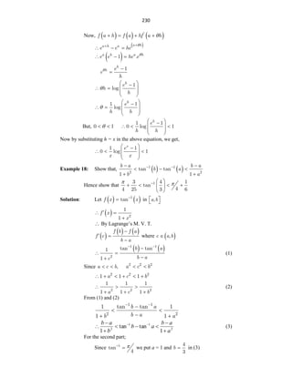
239. 239
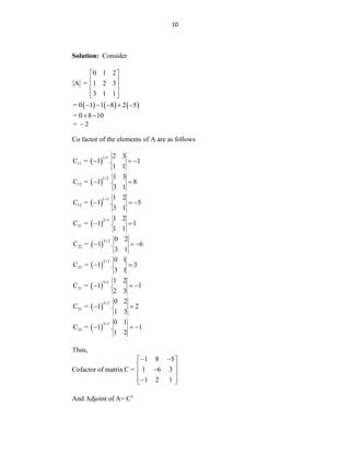
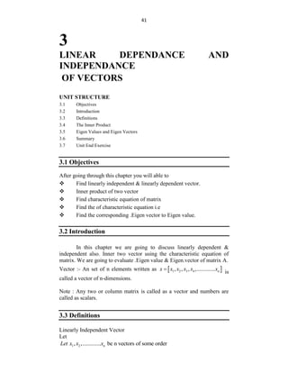
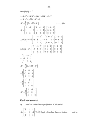
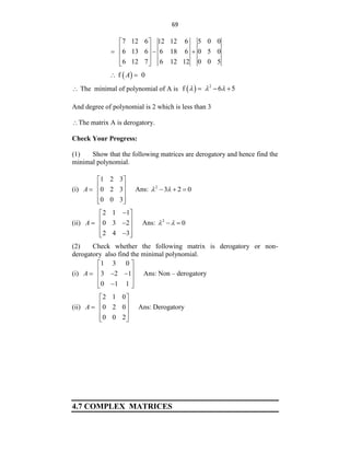
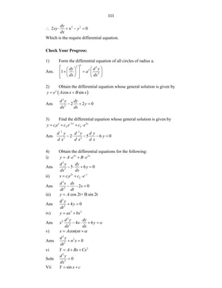
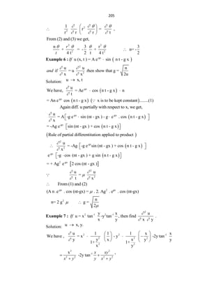
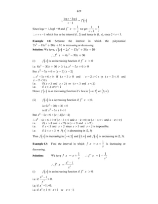
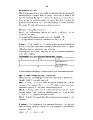
Fig. 13.1: f(x) = x, x (0, 1) Fig. 13.2 f(x) = x 3
, x 
If f is a continuous function defined on a closed and bounded interval
[a,b], then f has both a minimum and a maximum value on the interval
[a,b]. This is called the extreme value theorem and its proof is beyond the
scope of our course.
Look at the graph of some function f (x) in Fig. 13.3.
Fig. 13.3
Note that at x = x0 , the point A on graph is not an absolute maximum
because f(x2) > f(x0). But if we consider the interval (a,b), then f has a
maximum value at x = x0 in the interval (a,b). Point A is a point of local
maximum of f. Similarly f has a local minimum at point B.
Definition : Suppose f is a function defined on an intervals I. f is said to
have a local (relative) maximum at c I if there is a positive number h
such that for each x I for which c – h < x < c + h, x c
 we have f(x) >
f(c).
Definition : Suppose f is a function defined on an interval I. f is said to
have a local (relative) minimum at c I if there is a positive number h
such that for each xI for which c – h < x < c + h, x c
 we have f(x) <
f(c).
Again Fig. 13.4 suggest that at a relative extreme the derivative is either
zero or undefined. We call the x–values at these special points as critical
numbers.

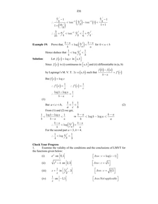
240. 240
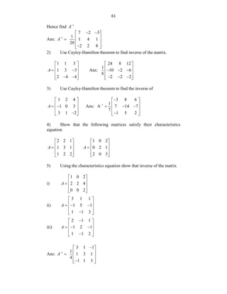
Fig 13.4
Definition :
If f is defined at c, then c is called a critical number if f if f ' (c) = 0 or f’ is
not defined at c. The following theorem which we state without proof tells
us that relative extreme can occur only at critical points.
Theorem: If f has a relative minimum or relative maximum at x= c, then c
is a critical number of f.
If f is a continuous function on interval [a,b], then the absolute extrema of
f occur either at a critical number or at the end points a and b. By
comparing the values of f at these points we can find the absolute
maximum or absolute minimum of f on [a, b].
Example 2 : Find the absolute maximum and minimum of the following
functions in the given interval. (i) f(x) = x2
on [–3, 3] (ii) f(x) = 3x4
– 4x3
on [–1, 2]
Solution : (i) f(x) = x2
, x [–3,3]
Differentiating w.r.t. x., we get f´(x) = 2x
To obtain critical numbers we set f´(x) = 0. This gives 2x = 0 or x = 0
which lies in the interval (–3,3).
Since f ' is defined for all x, we conclude that this is the only critical
number of f.
Let us now evaluate f at the critical number and at the end of points of [–
3,3].
f (–3) = 9
f (0) = 0
f (3) = 9
This shows that the absolute maximum of f on [–3,3] is f (–3) = f(3) = 9
and the absolute minimum is f (0) = 0
(ii) f(x) = 3x4
– 4x3
x [–1, 2] f´(x) = 12x3
– 12 x
To obtain critical numbers, we set f’ (x) = 0 or 12x3
– 12 x = 0 which
implies x = 0 or x = 1.
Both these values lie in the interval (–1, 2)
Let us now evaluate f at the critical number and at the end points of [–1,2]
f (–1) = 7
f (0) = 0
f (1) = –1
f (2) = 16
This shows that the absolute maximum 16 of f occurs at x = 2 and the
absolute minimum – 1 occurs at x = 1.

241. 241
First Derivative Test
How do we know whether f has a local maximum or a local minimum at a
critical point c ? we shall study two tests to decide whether a critical point
c is a point of local maxima or local minima. We begin with the following
result which is known as first derivative test. This result is stated without
any proof.
Theorem : Let c be a critical point for f, and suppose that f is continuous
at c and differentiable on some interval I containing c, except possibly at c
itself. Then
(i) if f´ changes from positive to negative at c, that is, if there exists some h
> 0 such that c – h < x < c, implies f´(x) > 0 and c < x < c + h implies f´(x)
< 0, then f has a local maximum at c.
(ii) if f´ changes sign from negative to positive at c, that is, if there exists
some h > 0 such that c – h < x < c implies f´(x) < 0 and c < x < c + h
implies f´(x) > 0 then f has a local minimum at c.
(iii) if f´(x) > 0 or if f´(x) < 0 for every x in I except x = c then f (c) is not a
local extremum of f.
Fig 13.5 Fig 13.6
As an illustration of ideas involved, imagine a blind person riding in a car.
If that person could feel the car travelling uphill then downhill, he or she
would know that the car has passed through a high point of the highway.
Essentially, the sign of derivative f '(x) indicates whether the graph goes
uphill or downhill. Therefore, without actually seeing the picture we can
deduce the right conclusion in each case. We summarize the first
derivative test for local maxima and minima as following:
First Derivative Test for Local Maxima and Minima
Let c be a critical number of f i.e., f´(c) = 0
If f´(x) changes sign from positive to negative at c then f (c) is a local
maximum. See fig 13.7. If f´(x) changes sign from negative to positive at c
then f(c) is a local minimum. See fig 13.8.
Note : f´(x) does not change, sign at c, then f(c) is neither a local
maximum nor local minimum.

242. 242
Fig 13.7
Fig 13.8
Example 3: Find the local (relative) extrema of the following functions :
(i) f (x) = 2x 3
+ 3x 2
– 12x +7 (ii) f (x) = 2
1
2
x 
(iii) f (x) = x.e x
Solution
(i) f is continuous and differentiable on R, the set of real numbers.
Therefore, the only critical values of f will be the solutions of the equation
f´(x) = 0.
Now, f´(x) = 2
6 6 12
x x
  = 6( 2)( 1)
x x
 
Setting f´(x) = 0 we obtain x = – 2, 1
Thus, x = –2 and x = 1 are the only critical numbers of f. Figure 13.9
shows the sign of derivative f´ in three intervals. From Figure 13.9 it is
clear that if x < –2, f´(x) > 0; if
–2 < x < 1, f´(x) < 0 and if x > 1, f´(x) > 0.
Fig 13.9
Using the first derivative test we conclude that f (x) has a local maximum
at x = – 2 and f (x) has local minimum at x = 1.
Now, f (–2) – 2 = 2(– 2) 3
+3(– 2) 2
– 12(–2) + 7 = –16 + 12 + 24 + 7 = 27
is the value of local maximum at x = – 2 and f (1) = 2 + 3 – 12+ 7 = 0 is
the value of local minimum at x = 1.
(ii) Since x 2
+ 2 is a polynomial and x 2
+ 2  0 is continuous and
differentiable on R, the set of real numbers. Therefore, the only critical
values of f (x) = 2
1
2
x 
will be the solutions of the equation f '(x) = 0.

243. 243
Setting f´(x) = 0 we obtain x = 0. Thus, x = 0 is the only critical number of
f. Figure 13.10 shows the sign of derivative in two intervals.
Now 2 2
(
( )
)
2
2x
f x
x




Setting f´(x) = 0 we obtain x = 0. Thus, x = 0 is the only critical number of
f. Figure 24 shows the sign of derivative in two intervals.
Fig. 13.10
From Figure 13.10 it is clear that f '(x) > 0 if x < 0 and f '(x) < 0 if x > 0.
Using the first derivative test, we conclude that f(x) has a local maximum
at x = 0.
Now since 2
1 1
(0)
2
0 2
f

  the value of the local maximum at x = 0 is
1/2.
(iii) Since x and e x
are continuous and differentiable on R, ( ) x
f x xe
 is
continuous and differentiable on R.
Therefore, the only critical values of f will be solutions of f´ (x) = 0.
Now, ( ) 1 ( 1)
x x x
f x xe e x e
    
Since 0,
x
x
e    , f´(x) = 0 gives x = –1. Thus, x = –1 is the only
critical number of f.
The figure below shows the sign of derivative f´ in two intervals :
It is clear that f´(x) < 0 if
x < –1 and f ´(x) > 0 if x > –1
Using the first derivative test
we conclude that f(x) has a
local minimum at x = –1 and
the value of local minimum
is
f (–1) = –1/e.

244. 244
Second Derivative Test
The first derivative test is very useful for finding the local maxima and
local minima of a function. But it is slightly cumbersome to apply as we
have to determine the sign of f ' around the point under consideration.
However, we can avoid determining the sign of derivative f ' around the
point under consideration, say c, if we know the sign of second derivative
f at point c. We shall call it as the second derivative test.
Theorem : (Second Derivative Test)
Let f(x) be a differentiable function on I and let c I. Let f ´ (x) be
continuous at c. Then
1. c is a point of local maximum if both f '(c) = 0 and f (c) < 0.
2. c is a point of local minimum if both f '(c) = 0 and f (c) > 0.
Remark : If f´(c) = 0 and f´´(c) = 0, then the second derivative test fails. In
this case, we use the first derivative test to determine whether c is a point
of local maximum or a point of a local minimum.
We summarize the second – derivative test for local maxima and minima
in the following table.
Second Derivative Test for Local Maxima and Minima
( )
f c
 ( )
f c
 ( )
f c
0 + Local Minimum
0 - Local Maximum
0 0 Test Fails
We shall adopt the following step to determine local maxima and minima.
Steps to find Local Maxima and Local Minima
The function f is assumed to posses the second derivative on the interval I.
Step 1 : Find f ' (x) and set it equal to 0.
Step 2 : Solve f ' (x) = 0 to obtain the critical numbers of f. Let the
solution of this equation be α, ………. We shall consider only those
values of x which lie in I and which are not end points of I.
Step 3 : Evaluate f ´ (α) If f (α) < 0, f (x) has a local maximum at x = α and
its value if f (α) If f (α) > 0, f (x) has a local minimum at x = α and its value
if f (α) If f (α) = 0, apply the first derivative test.
Step 4 : If the list of values in Step 2 is not exhausted, repeat step 3, with
that value.
Example 4: Find the points of local maxima and minima, if any, of each
of the following functions. Find also the local maximum values and local
minimum values.
(i) f (x) = 3 2
6 9 1
x
x x
   , x

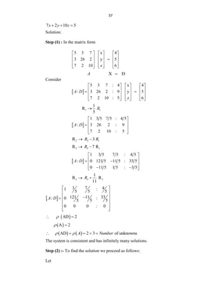
245. 245
(ii) f(x) = 3 2 2
2 ( 0),
x ax a x a x
   
Solution:
(i) f ´ (x) = 2
3 12 9
x x
  = 3( 1)( 3)
x x
 
To obtain critical number of f, we set f ´ (x) = 0 this yields x = 1, 3.
Therefore, the critical number of f are x = 1, 3.
Now f ´ (x) = 6x – 12 = 6(x – 2)
We have f ´ (1) = 6(1 – 2) = – 6 < 0 and f (3) = 6(3 – 2) = 6 > 0.
Using the second derivative test, we see that f (x) has a local maximum at
x = 1 and a local minimum at x = 3. The value of local maximum at x = 1 is f
(1) = 1– 6+ 9 +1 = 5 and the value of local minimum at x = 3 is
f (3) = 33
– 6(3)2
+ 9(3) + 1 = 27 – 54 + 27 + 1 = 1.
(ii) We have f(x) = 3 2 2
2 ( 0)
x ax a x a
  
Thus, 2 2
( ) 3 4 (3 )( )
ax a x a
f x x x a
      
As f '(x) is defined for each x R, to obtain critical number of f we set
f '(x) = 0.
This yields x = a/3 or x = a.
Therefore, the critical numbers of f and a/3 and a. Now, ( )
f a
 = 6x – 4a.
We have ( / 3) 6( / 3) 4 2 0
f a a a a
     
and ( ) 6 4 2 0
f a a a a
    
Using the second derivative test, we see that f(x) has a local maximum at x
= a/3 and a local minimum at x = a.
The value of local maximum at / 3
x a
 is 3
4
( / 3)
27
f a a
 and the value
of local minimum at x = a is ( ) 0
f a  .
Check Your Progress
1. Find the absolute maximum and minimum of the following functions in
the given intervals.
(i) f(x) = 4 – 7 x + 3 on [–2, 3]
(ii) f(x) =
3
2
x
x 
on [–1,1]
2. Using first derivative test find the local maxima and minima of the
following functions.
(i) 3
( ) 12
f x x x
  (ii)
2
( ) , 0
2
x
f x x
x
  
3. Use second derivative test to find the local maxima and minima of the
following functions.
(i) 3 2
( ) 2 1,
f x x x x x
     (ii) ( ) 2 1 , 1
f x x x x
   

246. 246
13.5 LET US SUM UP
The chapter is, as suggested by the title, on applications of differential
calculus. In section 13.4, methods for finding out (local) maxima and
minima, are discussed and explained with examples.