INTRODUCTION TO SELECTION SORT AND WORKING OF SELECTION SORT TO WATCH VIDEO: https://youtu.be/RlLn7tMiD3g TO DOWNLOAD PDF: https://computerassignmentsforu.blogspot.com/p/classxiiselectionsort.html

1. LIST IN PYTHON
SELECTION SORT
CLASS: XII
COMPUTER SCIENCE(083)
PART-6

2. WHAT IS SELECTION SORT?
The Selection sort is based on the idea of finding the minimum or maximum
element in an unsorted array and then putting it in its correct position in a sorted
LIST
How Selection Sort Works?
Step 1: Select the first element of the list and set the first element as minimum
Step 2: Compare minimum with the next element. If the next element is smaller than
minimum, assign the next element as minimum. This process goes on until the last
element.
Step 3: After each iteration, minimum is placed in the front of the unsorted list.
Step 4: Step 1 to 3 are repeated until all the elements are placed at their correct
positions.

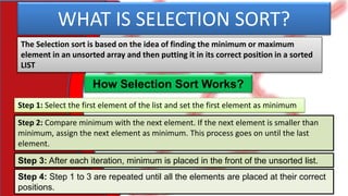
3. How Selection Sort Works?
0 1 2 3 4
20 12 10 15 2
Let Us Understand With The Help Of Example:
no=
These are unsorted number and we need to sort them with the help of selection sort
20 12 10 15 2
Step 1: initialize the list with numbers as shown below:
no=[20,12,10,15,2]

4. Step 2: Declare variable K and store the
length of list.
no=[20,12,10,15,2]
K=len(no)
0 1 2 3 4
20 12 10 15 2
no=
K=5
Step 4: Start the outer loop x from 0 to K-1
for x in range(0,K):
x=0 k
Step 5: Start the inner loop y from 0 to K-1
Step 5: before starting inner loop store minimum =x the index number
min=x
for y in range(x+1,k):
y=x+1=0+1=1

5. Step 2: Declare variable K and store the length of list.
no=[20,12,10,15,2]
K=len(no)
0 1 2 3 4
20 12 10 15 2
no=
K=5
Step 4: Start the outer loop x from 0 to K-1
for x in range(0,K):
x=0 k
Step 5: Start the inner loop y from 0 to K-1
Step 5: before starting inner loop store minimum =x the index number
min=x
for y in range(0+1,k):
Step 6: Start if condition inside inner loop to check no[min] value is greater than no[y] or
not.
if no[min]> no[y]:
Step 7: if condition TRUE than overwrite the minimum value with y
min=y

6. Step 2: Declare variable K and store the length of list.
no=[20,12,10,15,2]
K=len(no)
0 1 2 3 4
20 12 10 15 2
no=
K=5
Step 4: Start the outer loop x from 0 to K-1
for x in range(0,K):
x=0 k
Step 5: Start the inner loop y from 0 to K-1
Step 5: before starting inner loop store minimum =x the index number
min=x
for y in range(0+1,k):
Step 6: Start if condition inside inner loop to check no[min] value is greater than no[y] or not.
if no[min]> no[y]:
Step 7: if condition TRUE than overwrite the minimum value with y
min=y
Step 8:Every time when inner loop finished swapping starts before outer loop move to next step
tmp=no[min]
no[min]=no[x]
no[x]=tmp

7. Step 2: Declare variable K and store the length of list.
no=[20,12,10,15,2]
K=len(no) 0 1 2 3 4
20 12 10 15 2
no=
K=5
Step 4: Start the outer loop x from 0 to K-1
for x in range(0,K):
x=0 k
Step 5: Start the inner loop y from 0 to K-1
Step 5: before starting inner loop store minimum =x the index number
min=x
for y in range(0+1,k):
Step 6: Start if condition inside inner loop to check no[min] value is greater than no[y] or not.
if no[min]> no[y]:
Step 7: if condition TRUE than overwrite the minimum value with y
min=y
Step 8:Every time when inner loop finished swapping starts before outer loop move to next step
tmp=no[min]
no[min]=no[x]
no[x]=tmp
Step 9: Display the final result
print(no)

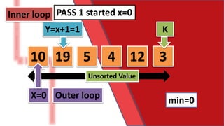
8. no=[10,19,5,4,12,3]
K=len(no)
for x in range(0,K):
min = x
for y in range(x + 1, K):
if no[min]> no[y]:
min = y
temp= no[min];
no[min] = no[x]
no[x]=temp
print("Pass: ",x+1,"=",no)
print("Final List:",no)
SELECTION SORT FULL CODE:
Inner loop
Outer loop
Outer loop

9. 10 19 5 4 12 3
PASS 1 started x=0
Unsorted Value
Y=x+1=1 K
X=0
Inner loop
Outer loop
min=0

10. SELECTION SORT:
no=[10,19,5,4,12,3]
K=len(no)
for x in range(0,K):
min = x
for y in range(x + 1, K):
if no[min]> no[y]:
min = y
temp= no[min];
no[min] = no[x]
no[x]=temp
print("Pass: ",x+1,"=",no)
print("Final List:",no)
10 19 5 4 12 3no=
0 1 2 3 4 5
x=0 min=x
K
Outer loop [this is pass 1]
Inner loop start where y starts from x+1 to K
y=1 10 19 5 4 12 3 min=0x=0
y=1
K=6(less than 6)
if 10>19 FALSE min value remain same
min=0

11. SELECTION SORT:
no=[10,19,5,4,12,3]
K=len(no)
for x in range(0,K):
min = x
for y in range(x + 1, K):
if no[min]> no[y]:
min = y
temp= no[min];
no[min] = no[x]
no[x]=temp
print("Pass: ",x+1,"=",no)
print("Final List:",no)
10 19 5 4 12 3no=
0 1 2 3 4 5
x=0 min=x
K
Outer loop [this is pass 1]
y=1
y=2
10 19 5 4 12 3
min=0x=0
y=2
K=6(less than 6)
if 10>5 TRUE min value change to 2
min=0
10 19 5 4 12 3

12. SELECTION SORT:
no=[10,19,5,4,12,3]
K=len(no)
for x in range(0,K):
min = x
for y in range(x + 1, K):
if no[min]> no[y]:
min = y
temp= no[min];
no[min] = no[x]
no[x]=temp
print("Pass: ",x+1,"=",no)
print("Final List:",no)
10 19 5 4 12 3no=
0 1 2 3 4 5
x=0 min=x
K
Outer loop [this is pass 1]
y=1
y=2
y=3
10 19 5 4 12 3
min=2x=0
K=6(less than 6)
if 5>4 TRUE min value change to 3
10 19 5 4 12 3
y=3min=2
10 19 5 4 12 3

13. SELECTION SORT:
no=[10,19,5,4,12,3]
K=len(no)
for x in range(0,K):
min = x
for y in range(x + 1, K):
if no[min]> no[y]:
min = y
temp= no[min];
no[min] = no[x]
no[x]=temp
print("Pass: ",x+1,"=",no)
print("Final List:",no)
10 19 5 4 12 3no=
0 1 2 3 4 5
x=0 min=x
K
Outer loop [this is pass 1]
y=1
y=2
y=3
y=4
10 19 5 4 12 3
min=3x=0
K=6(less than 6)
if 4>12 FALSE min value remain 3
10 19 5 4 12 3
y=4min=3
10 19 5 4 12 3
10 19 5 4 12 3

14. SELECTION SORT:
no=[10,19,5,4,12,3]
K=len(no)
for x in range(0,K):
min = x
for y in range(x + 1, K):
if no[min]> no[y]:
min = y
temp= no[min];
no[min] = no[x]
no[x]=temp
print("Pass: ",x+1,"=",no)
print("Final List:",no)
10 19 5 4 12 3no=
0 1 2 3 4 5
x=0 min=x
K
Outer loop [this is pass 1]
y=1
y=2
y=3
y=4
y=5
10 19 5 4 12 3
min=3x=0
K=6(less than 6)
if 4>3 TRUE min value change to 5
10 19 5 4 12 3
y=5min=3
10 19 5 4 12 3
10 19 5 4 12 3
10 19 5 4 12 3

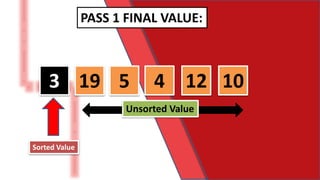
15. SELECTION SORT:
no=[10,19,5,4,12,3]
K=len(no)
for x in range(0,K):
min = x
for y in range(x + 1, K):
if no[min]> no[y]:
min = y
temp= no[min];
no[min] = no[x]
no[x]=temp
print("Pass: ",x+1,"=",no)
print("Final List:",no)
10 19 5 4 12 3no=
0 1 2 3 4 5
x=0 min=x
K
Outer loop [this is pass 1]
y=1
y=2
y=3
y=4
y=5
10 19 5 4 12 3
min=5x=0
Now Swapping start
tmp= 3 temp=no[min]
10 19 5 4 12 3
min=5
10 19 5 4 12 3
10 19 5 4 12 3
10 19 5 4 12 3
x=0
swap
Inner loop finish
no[min]=no[x]no[5]= 10
no[0]= 3 no[x]=temp1019 5 4 123
Pass 1 Final value:

16. 1019 5 4 123
PASS 1 FINAL VALUE:
Sorted Value
Unsorted Value

17. 1019 5 4 123
PASS 2 STARTS Where X=1
Sorted Value
Y=x+1=1+1=2 K
X=1
Inner loop
Outer loop
min=1

18. SELECTION SORT:
no=[10,19,5,4,12,3]
K=len(no)
for x in range(0,K):
min = x
for y in range(x + 1, K):
if no[min]> no[y]:
min = y
temp= no[min];
no[min] = no[x]
no[x]=temp
print("Pass: ",x+1,"=",no)
print("Final List:",no)
3 19 5 4 12 10no=
0 1 2 3 4 5
x=1 min=x
K
Outer loop [this is pass 2]
Inner loop start where y starts from x+1 to K
y=2 3 19 5 4 12 10 min=1x=1
y=2
K=6(less than 6)
if 19>5 TRUE min value Change 2
min=1

19. SELECTION SORT:
no=[10,19,5,4,12,3]
K=len(no)
for x in range(0,K):
min = x
for y in range(x + 1, K):
if no[min]> no[y]:
min = y
temp= no[min];
no[min] = no[x]
no[x]=temp
print("Pass: ",x+1,"=",no)
print("Final List:",no)
3 19 5 4 12 10no=
0 1 2 3 4 5
x=0 min=x
K
Outer loop [this is pass 1]
y=2
y=3
3 19 5 4 12 10
min=2x=1
y=3
K=6(less than 6)
If 5>4 TRUE min value change to 3
min=2
3 19 5 4 12 10

20. SELECTION SORT:
no=[10,19,5,4,12,3]
K=len(no)
for x in range(0,K):
min = x
for y in range(x + 1, K):
if no[min]> no[y]:
min = y
temp= no[min];
no[min] = no[x]
no[x]=temp
print("Pass: ",x+1,"=",no)
print("Final List:",no)
3 19 5 4 12 10no=
0 1 2 3 4 5
x=0 min=x
K
Outer loop [this is pass 1]
y=2
y=3
y=4
3 19 5 4 12 10
min=3x=1
K=6(less than 6)
if 4>12 FALSE min value remain same
3 19 5 4 12 10
y=4min=3
3 19 5 4 12 10

21. SELECTION SORT:
no=[10,19,5,4,12,3]
K=len(no)
for x in range(0,K):
min = x
for y in range(x + 1, K):
if no[min]> no[y]:
min = y
temp= no[min];
no[min] = no[x]
no[x]=temp
print("Pass: ",x+1,"=",no)
print("Final List:",no)
3 19 5 4 12 10no=
0 1 2 3 4 5
x=0 min=x
K
Outer loop [this is pass 1]
y=2
y=3
y=4
y=5
3 19 5 4 12 10
min=3x=1
K=6(less than 6)
If 4>10 FALSE min value remain same
3 19 5 4 12 10
y=5min=3
3 19 5 4 12 10
3 19 5 4 12 10

22. SELECTION SORT:
no=[10,19,5,4,12,3]
K=len(no)
for x in range(0,K):
min = x
for y in range(x + 1, K):
if no[min]> no[y]:
min = y
temp= no[min];
no[min] = no[x]
no[x]=temp
print("Pass: ",x+1,"=",no)
print("Final List:",no)
3 19 5 4 12 10no=
0 1 2 3 4 5
x=0 min=x
K
Outer loop [this is pass 1]
y=2
y=3
y=4
y=5
3 19 5 4 12 10
min=3x=1
Now Swapping start
tmp= 4 temp=no[min]
3 19 5 4 12 10
min=3
3 19 5 4 12 10
3 19 5 4 12 10
x=1
swap
Inner loop finish
no[min]=no[x]no[3]= 19
no[1]= 4 no[x]=temp101954 123
Pass 2 Final value:

23. 101954 123
PASS 2 FINAL VALUE:
Unsorted Value
Sorted Value

24. 101954 123
PASS 3 STARTS Where X=2
Sorted Value
Y=x+1=3 K
X=2
Inner loop
Outer loop

25. SELECTION SORT:
no=[10,19,5,4,12,3]
K=len(no)
for x in range(0,K):
min = x
for y in range(x + 1, K):
if no[min]> no[y]:
min = y
temp= no[min];
no[min] = no[x]
no[x]=temp
print("Pass: ",x+1,"=",no)
print("Final List:",no)
3 1954 12 10no=
0 1 2 3 4 5
x=2 min=x
K
Outer loop [this is pass 3]
Inner loop start where y starts from x+1 to K
y=3 3 1954 12 10 min=2x=2
y=3
K=6(less than 6)
If 5>19 FALSE min value remain same
min=2

26. SELECTION SORT:
no=[10,19,5,4,12,3]
K=len(no)
for x in range(0,K):
min = x
for y in range(x + 1, K):
if no[min]> no[y]:
min = y
temp= no[min];
no[min] = no[x]
no[x]=temp
print("Pass: ",x+1,"=",no)
print("Final List:",no)
3 1954 12 10no=
0 1 2 3 4 5
x=0 min=x
K
Outer loop [this is pass 3]
y=3
y=4
3 1954 12 10
min=2x=2
y=4
K=6(less than 6)
If 5>12 FALSE min value remain same
min=2
3 1954 12 10

27. SELECTION SORT:
no=[10,19,5,4,12,3]
K=len(no)
for x in range(0,K):
min = x
for y in range(x + 1, K):
if no[min]> no[y]:
min = y
temp= no[min];
no[min] = no[x]
no[x]=temp
print("Pass: ",x+1,"=",no)
print("Final List:",no)
3 1954 12 10no=
0 1 2 3 4 5
x=0 min=x
K
Outer loop [this is pass 3]
y=3
y=4
y=5
3 1954 12 10
min=2x=2
K=6(less than 6)
If 5>10 FALSE min value remain same
3 1954 12 10
y=5min=2
3 1954 12 10

28. SELECTION SORT:
no=[10,19,5,4,12,3]
K=len(no)
for x in range(0,K):
min = x
for y in range(x + 1, K):
if no[min]> no[y]:
min = y
temp= no[min];
no[min] = no[x]
no[x]=temp
print("Pass: ",x+1,"=",no)
print("Final List:",no)
3 1954 12 10no=
0 1 2 3 4 5
x=0 min=x
K
Outer loop [this is pass 3]
y=3
y=4
y=5
min=2x=2
Now Swapping start
tmp= 5 temp=no[min]
3 1954 12 10
min=2
3 1954 12 10
3 1954 12 10
x=2swap
Inner loop finish
no[min]=no[x]no[2]= 5
no[2]= 5 no[x]=temp101954 123
Pass 3 Final value:

29. 101954 123
PASS 3 FINAL VALUE:
Unsorted Value
Sorted Value

30. 101954 123
PASS 4 STARTS Where X=3
Sorted Value
Y=x+1=4 K
X=3
Inner loop
Outer loop

31. SELECTION SORT:
no=[10,19,5,4,12,3]
K=len(no)
for x in range(0,K):
min = x
for y in range(x + 1, K):
if no[min]> no[y]:
min = y
temp= no[min];
no[min] = no[x]
no[x]=temp
print("Pass: ",x+1,"=",no)
print("Final List:",no)
3 1954 12 10no=
0 1 2 3 4 5
x=3 min=x
K
Outer loop [this is pass 4]
Inner loop start where y starts from x+1 to K
y=4 3 1954 12 10 min=3x=3
y=4
K=6(less than 6)
If 19>12 TRUE min value change to 4
min=3

32. SELECTION SORT:
no=[10,19,5,4,12,3]
K=len(no)
for x in range(0,K):
min = x
for y in range(x + 1, K):
if no[min]> no[y]:
min = y
temp= no[min];
no[min] = no[x]
no[x]=temp
print("Pass: ",x+1,"=",no)
print("Final List:",no)
3 1954 12 10no=
0 1 2 3 4 5
x=3 min=x
K
Outer loop [this is pass 4]
y=4
y=5
3 1954 12 10
min=4x=3
y=5
K=6(less than 6)
If 12>10 TRUE min value change to 5
min=4
3 1954 12 10

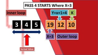
33. SELECTION SORT:
no=[10,19,5,4,12,3]
K=len(no)
for x in range(0,K):
min = x
for y in range(x + 1, K):
if no[min]> no[y]:
min = y
temp= no[min];
no[min] = no[x]
no[x]=temp
print("Pass: ",x+1,"=",no)
print("Final List:",no)
3 1954 12 10no=
0 1 2 3 4 5
x=3 min=x
K
Outer loop [this is pass 4]
y=4
y=5
min=5
x=3
Now Swapping start
tmp= 10 temp=no[min]
min=5
3 1954 12 10
3 1954 12 10
x=3
swap
Inner loop finish
no[min]=no[x]no[5]= 19
no[3]= 10 no[x]=temp191054 123
Pass 4 Final value:

34. 10 1954 123
PASS 4 FINAL VALUE:
Unsorted Value
Sorted Value

35. 10 1954 123
PASS 5 STARTS Where X=4
Sorted Value
Y=x+1=5
K
x=4
Inner loop
Outer loop

36. SELECTION SORT:
no=[10,19,5,4,12,3]
K=len(no)
for x in range(0,K):
min = x
for y in range(x + 1, K):
if no[min]> no[y]:
min = y
temp= no[min];
no[min] = no[x]
no[x]=temp
print("Pass: ",x+1,"=",no)
print("Final List:",no)
3 1054 12 19no=
0 1 2 3 4 5
x=4 min=x
K
Outer loop [this is pass 5]
Inner loop start where y starts from x+1 to K
y=5 3 1054 12 19 min=4x=4
y=5
K=6(less than 6)
If 12>19 FALSE min value remain same
min=4

37. SELECTION SORT:
no=[10,19,5,4,12,3]
K=len(no)
for x in range(0,K):
min = x
for y in range(x + 1, K):
if no[min]> no[y]:
min = y
temp= no[min];
no[min] = no[x]
no[x]=temp
print("Pass: ",x+1,"=",no)
print("Final List:",no)
3 1054 12 19no=
0 1 2 3 4 5
x=3 min=x
K
Outer loop [this is pass 4]
y=5
min=4
x=4
Now Swapping start
tmp= 12 temp=no[min]
min=4
3 1054 12 19
x=4
swap
Inner loop finish
no[min]=no[x]no[4]= 12
no[4]= 12 no[x]=temp191054 123
Pass 5 Final value:

38. 10 1954 123
PASS 5 FINAL VALUE:
Unsorted Value
Sorted Value

39. 10 1954 123
FINAL RESULT OF SELECTION SORT:
Sorted Value