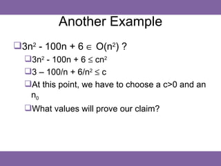
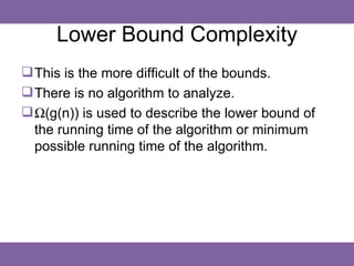
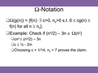
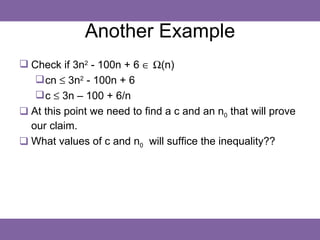
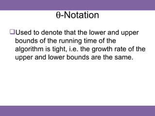
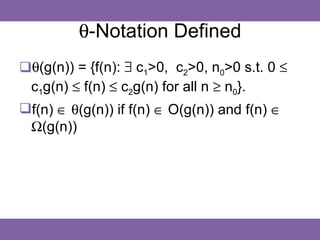
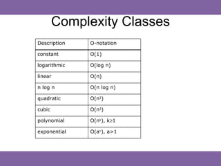
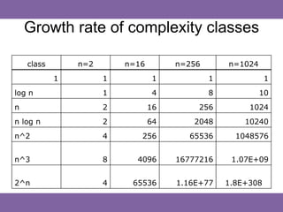
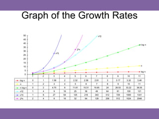
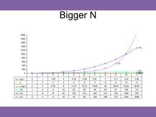
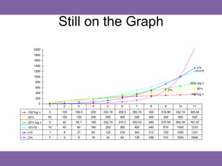
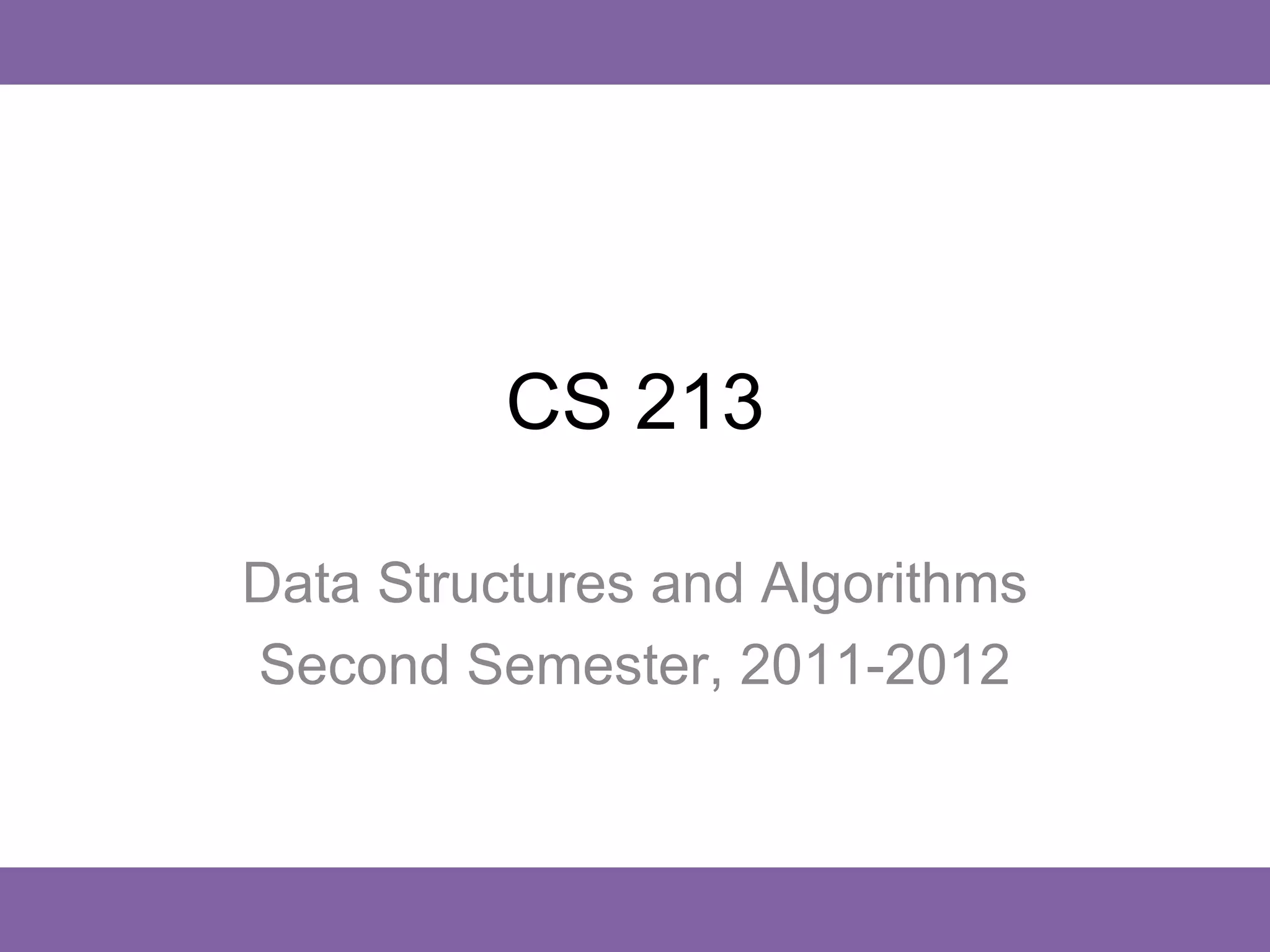
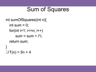
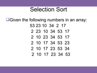
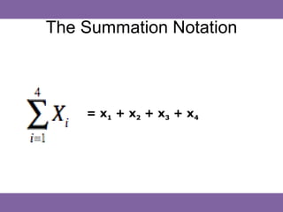
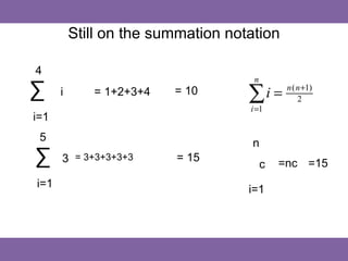
The document covers concepts related to algorithms and data structures taught in a CS213 course, including a function for calculating the sum of squares and the selection sort algorithm. It discusses time complexity analysis, including lower and upper bounds, the goal of aligning these bounds, and introduces big O, ω, and θ notations for analyzing algorithm performance. Examples and complexity classes for different growth rates are also provided to illustrate the concepts.

1. CS 213
Data Structures and Algorithms
Second Semester, 2011-2012

2. Sum of Squares
int sumOfSquares(int n){
int sum = 0;
for(int i=1; i<=n; i++)
sum = sum + i*i;
return sum;
}
 T(n) = 5n + 4

3. Selection Sort
Given the following numbers in an array:
53 23 10 34 2 17
2 23 10 34 53 17
2 10 23 34 53 17
2 10 17 34 53 23
2 10 17 23 53 34
2 10 17 23 34 53

4. Still on Selection Sort
void selectionSort(int A[], int n){
for(int i=0; i<n; i++){
int min = i;
for(int j=i+1; j<n; j++){
if(A[j] < A[min])
min = j;
What is this function’s T(n)? What
} we need is to compute for T(n)
int temp = A[i]; from the inner loop going
A[i] = A[min]; outwards.
A[min] = temp;
We need to use the summation
} notation to solve the T(n).
}

5. The Summation Notation
= x1 + x2 + x3 + x4

6. Still on the summation notation
4
n
∑ i = 1+2+3+4 = 10
∑i = n ( n +1)
2
i =1
i=1
5
n
∑ 3 = 3+3+3+3+3 = 15
∑c =nc =15
i=1 i=1

7. Exercise
 for(int i=1; i<=5; i++) cout<<endl;
 for(int i=1; i<=n; i++) cout<<endl;
 for(int i=3; i<=m; i++) cout<<endl;
 for(int i=1; i<=6; i++)
for(int j=1; j<=8; j++) cout<<endl;
 for(int i=1; i<=n; i++)
for(int j=1; j<=n; j++) cout<<endl;
 for(int i=1; i<=m; i++)
for(int j=1; j<=m; j++) cout<<endl;
 for(int i=1; i<=n; i++)
for(int j=i; j<=n; j++) cout<<endl;

8. Going back to the Selection Sort
void selectionSort(int A[], int n){
for(int i=0; i<n; i++){ n n n
int min = i;
for(int j=i+1; j<n; j++){ ∑ ∑ c =∑ c(n-i+1-1)
if(A[j] < A[min]) i=1 j=i+1 i=1
min = j;
} n n
int temp = A[i];
A[i] = A[min]; ∑ c(n-i) = c n-i∑
A[min] = temp; i=1 i=1
}
n n n
}
∑ n-i = ∑ n - ∑ i
i=1 i=1 i=1

9. Time Complexity
A function that maps problem size into the
time required to solve the problem.
Typically, we are interested in the inherent
complexity of computing the solution to
problems in a particular class.

10. Lower Bound
 We might want to know how fast we can sort a list of n
items, initially in an arbitrary order, regardless of the
algorithm used.
 What is sought here is the lower bound, L(n), on sorting,
a property of the sorting problem and not of any
particular algorithm.
 This says that no algorithm can do the job in fewer than
L(n) time units for arbitrary inputs.

11. Upper Bound
 We might also like to know how long it would
take to sort such list using a known algorithm
with a worst-case input.
 What is sought here is the upper bound, U(n),
which says that for arbitrary inputs we can
always sort in time at most U(n).

12. Goal of Time Complexity Analysis
 While there are apparently two complexity functions for
problems, L(n) and U(n), the ultimate goal is to make
these two bounds coincide.
 This is the optimal algorithm which has L(n) = U(n).
 For some of the problems, this goal has not been
realized yet!

13. Invitation
Consider this, CS 213, as you journey into
finding optimal solutions to classes of
problems!
Who knows, you might win a million
dollars ($$$) from Claymath Foundation!

14. Upper Bound Complexity
There are two ways in analyzing this
bound:
Counting instructions
Solving recurrences
Both are used to find the worst case of an
algorithm.

15. Big O-Notation (O(g(n)))
The O-notation is used to describe the
worst-case running time of an algorithm.
O(n) means that the growth of the running
time of the algorithm is a function of n.
O-notation computes for the upper bound.

16. O-Notation Defined
O(g(n)) = {f(n): ∃ c>0, n0>0 s.t. 0 ≤ f(n) ≤
cg(n) for all n ≥ n0}.
Example: Check if (n2/2) – 3n ∈ O(n2)
(n2/2) – 3n ≤ cn2
½ - 3/n ≤ c
Choosing c = ½, n0 = 6 proves the claim.

17. Another Example
3n2 - 100n + 6 ∈ O(n2) ?
3n2 - 100n + 6 ≤ cn2
3 – 100/n + 6/n2 ≤ c
At this point, we have to choose a c>0 and an
n0
What values will prove our claim?

18. Lower Bound Complexity
 This is the more difficult of the bounds.
 There is no algorithm to analyze.
 Ω(g(n)) is used to describe the lower bound of
the running time of the algorithm or minimum
possible running time of the algorithm.

19. Ω-Notation
Ω(g(n)) = {f(n): ∃ c>0, n0>0 s.t. 0 ≤ cg(n) ≤
f(n) for all n ≥ n0}.
Example: Check if (n2/2) – 3n ∈ Ω(n2)
cn2 ≤ (n2/2) – 3n
c ≤ ½ - 3/n
Choosing c = 1/14, n0 = 7 proves the claim.

20. Another Example
 Check if 3n2 - 100n + 6 ∈ Ω(n)
 cn ≤ 3n2 - 100n + 6
 c ≤ 3n – 100 + 6/n
 At this point we need to find a c and an n0 that will prove
our claim.
 What values of c and n0 will suffice the inequality??

21. θ-Notation
Used to denote that the lower and upper
bounds of the running time of the
algorithm is tight, i.e. the growth rate of the
upper and lower bounds are the same.

22. θ-Notation Defined
θ(g(n)) = {f(n): ∃ c1>0, c2>0, n0>0 s.t. 0 ≤
c1g(n) ≤ f(n) ≤ c2g(n) for all n ≥ n0}.
f(n) ∈ θ(g(n)) if f(n) ∈ O(g(n)) and f(n) ∈
Ω(g(n))

23. Complexity Classes
Description O-notation
constant O(1)
logarithmic O(log n)
linear O(n)
n log n O(n log n)
quadratic O(n2)
cubic O(n3)
polynomial O(nk), k≥1
exponential O(an), a>1

24. Growth rate of complexity classes
class n=2 n=16 n=256 n=1024
1 1 1 1 1
log n 1 4 8 10
n 2 16 256 1024
n log n 2 64 2048 10240
n^2 4 256 65536 1048576
n^3 8 4096 16777216 1.07E+09
2^n 4 65536 1.16E+77 1.8E+308

25. Graph of the Growth Rates
50 n^2
45
40
n log n
35
2^n
30
n^3
25
20
15
10 n
5
log n
0
1 2 3 4 5 6 7 8 9 10 11
log n 0 1 1.58 2 2.32 2.58 2.81 3 3.17 3.32 3.46
n 1 2 3 4 5 6 7 8 9 10 11
n log n 0 2 4.75 8 11.61 15.51 19.65 24 28.53 33.22 38.05
n^2 1 4 9 16 25 36 49 64 81 100 121
n^3 1 8 27 64 125 216 343 512 729 1000 1331
2^n 2 4 8 16 32 64 128 256 512 1024 2048

26. Bigger N
2000
1800
1600
1400
n^3
1200
1000
800
600
2^n
400
200
n^2
0 n log n
n n
log
1 2 3 4 5 6 7 8 9 10 11
log n 0 1 1.58 2 2.32 2.58 2.81 3 3.17 3.32 3.46
n 1 2 3 4 5 6 7 8 9 10 11
n log n 0 2 4.75 8 11.61 15.51 19.65 24 28.53 33.22 38.05
n^2 1 4 9 16 25 36 49 64 81 100 121
n^3 1 8 27 64 125 216 343 512 729 1000 1331
2^n 2 4 8 16 32 64 128 256 512 1024 2048

27. Still on the Graph
2000
1800
1600
1400
n^3
1200 10*n^2
1000
800 20*n log n
600 50*n
2^n
400 100*log n
200
0
1 2 3 4 5 6 7 8 9 10 11
100*log n 0 100 158.5 200 232.19 258.5 280.74 300 316.99 332.19 345.94
50*n 50 100 150 200 250 300 350 400 450 500 550
20*n log n 0 40 95.1 160 232.19 310.2 393.03 480 570.59 664.39 761.07
10*n^2 10 40 90 160 250 360 490 640 810 1000 1210
n^3 1 8 27 64 125 216 343 512 729 1000 1331
2^n 2 4 8 16 32 64 128 256 512 1024 2048