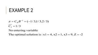
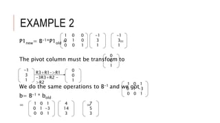
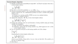
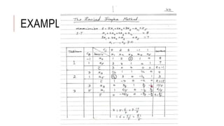
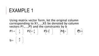
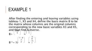
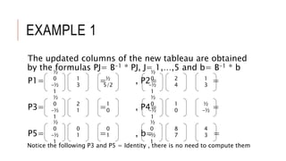
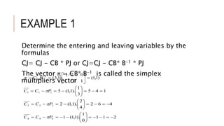
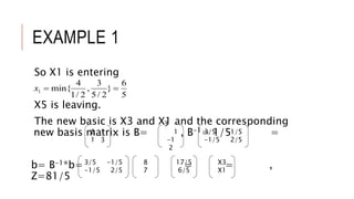
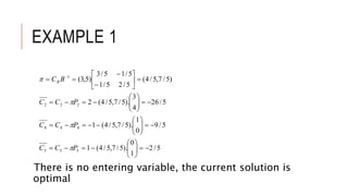
This document provides examples of using the revised simplex method to solve linear programming problems. Example 1 walks through applying the method step-by-step to a multi-variable problem. It shows setting up the initial tableau, finding the entering and leaving variables, and updating the basis matrix at each iteration until an optimal solution is reached. Example 2 solves a problem with artificial variables using the two-phase method. It demonstrates writing the problem in standard and canonical form, and iteratively choosing entering/leaving variables and updating the basis matrix over two iterations to find the optimal solution.

1. CHAPTER 08 – THE
REVISED SIMPLEX
METHOD
Operations research

3. EXAMPLE 1

4. EXAMPLE 1
Using matrix vector form, let the original column
corresponding to X1,…,X5 be denoted by column
vectors P1,…,P5 and the constraints by b
P1= P2= P3= P4= P5=
b=
1
3
2
4
2
1
1
0
0
1
8
7

5. EXAMPLE 1
After finding the entering and leaving variables using
tableau 1, X3 and X4, define the basis matrix B to be
the matrix whose columns are the original columns
corresponding to the new basic variables X3 and X5,
and then find B inverse.
B= =
B-1= ½ =
P3,P
5
2 0
1 1
1 0
-1
2
½
0
-½
1

6. EXAMPLE 1
The updated columns of the new tableau are obtained
by the formulas PJ= B-1 * PJ, J= 1,…,5 and b= B-1 * b
P1= = , P2= =
P3= = , P4= =
P5= = , b= =
Notice the following P3 and P5 = Identity , there is no need to compute them
½
0
-½
1
1
3
½
5/2
½
0
-½
1
2
4
1
3
½
0
-½
1
2
1
1
0
½
0
-½
1
½
-½
1
0
½
0
-½
1
0
1
0
1
½
0
-½
1
8
7
4
3

7. EXAMPLE 1
Determine the entering and leaving variables by the
formulas
CJ= CJ - CB * PJ or CJ=CJ - CB* B-1 * PJ
The vector π = CB* B-1 is called the simplex
multipliers vector
211
0
1
).1,1(1
462
4
2
).1,1(2
145
3
1
).1,1(5
)1,1(
12/1
02/1
)1,3(
444
222
111
1




























 
PCC
PCC
PCC
BCB





8. EXAMPLE 1
So X1 is entering
X5 is leaving.
The new basic is X3 and X1 and the corresponding
new basis matrix is B= , B-1= 1/5 =
b= B-1*b= = = ,
Z=81/5
5
6
}
2/5
3
,
2/1
4
min{1 x
2 1
1 3
3 -
1
-1
2
3/5 -1/5
-1/5 2/5
3/5 -1/5
-1/5 2/5
8
7
17/5
6/5
X3
X1

9. EXAMPLE 1
There is no entering variable, the current solution is
optimal
5/2
1
0
).5/7,5/4(1
5/9
0
1
).5/7,5/4(1
5/26
4
3
).5/7,5/4(2
)5/7,5/4(
5/25/1
5/15/3
)5,3(
555
444
222
1





























 
PCC
PCC
PCC
BCB





10. CHARACTERISTICS OF THE REVISED
SIMPLEX METHOD1. Any needed information can be obtained directly from the
original equations by knowing the inverse of the basis
matrix.
2. The inverse of the basis matrix can be obtained from the
original equations by knowing the current basic variables.
3. Finding the inverse of a matrix is usually considered time
consuming from computational viewpoint. Thus, this inverse
is obtained at each step by a simple pivot operation on the
previous inverse as follows:
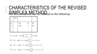
Example: Since are the initial basic variables, the
initial basis matrix is: and in any subsequent
tableau, the new column coefficients corresponding to
are obtained by pre multiplying by the inverse of
the current basis matrix. That is:
54 and xx
IPP ],[ 54
54 and xx 54 and PP
11
54
1
5
1
4
1
54 ],[],[],[




BIB
PPBPBPBPP

11. CHARACTERISTICS OF THE REVISED
SIMPLEX METHODThe second tableau can be reduced to the following:
211
0
1
).1,1(1
462
4
2
).1,1(2
145
3
1
).1,1(5
)1,1(
12/1
02/1
)1,3(
444
222
111
1




























 
PCC
PCC
PCC
BCB





12. CHARACTERISTICS OF THE REVISED
SIMPLEX METHODSo, is the new entering variable, and
Since this is the second component, the second current basic
variable, , is the leaving variable. This means that the pivot
column should be reduced to the column . To do
this, perform the following:
Multiply the second row by 2/5.
Multiply second row by -1/2 and add the result to first row.
Apply these two operations on current inverse and the vector b.
1x
5
6
}
2/5
3
,
2/1
4
min{
givesruleratiominimumtheand
3
4
7
8
12/1
02/1
2/5
2/1
3
1
12/1
02/1
1
1
1
1
1











































x
bBb
PBP
5x






2/5
2/1






1
0

13. CHARACTERISTICS OF THE REVISED
SIMPLEX METHODThe new tableau will be:
The new bfs is: ,5/81,5/6,5/17 13  zxx

14. EXAMPLE 2
Min Z= -3x1 + x2 + x3
S.T. x1 – 2x2 + x3 <= 11
-4x1+ x2 + 2x3 >= 3
2x1 – x3 = -1
If the problem have an artificial variables we solve it using by Big
M or by two phase method.

15. EXAMPLE 2
Write the problem in standard form
Min Z= -3x1 + x2 + x3
S.T. x1 – 2x2 + x3 + x4 = 11, Slack
-4x1 + x2 +2x3 – x5 = 3, Surplus
-2x1 + x3 = 1

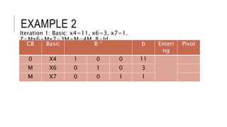
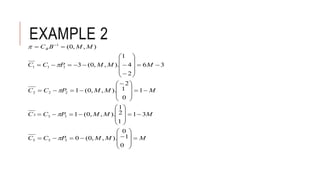
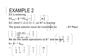
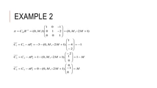
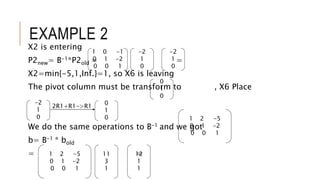
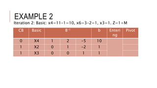
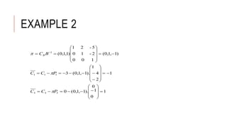
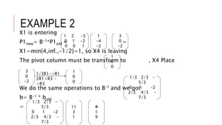
16. EXAMPLE 2
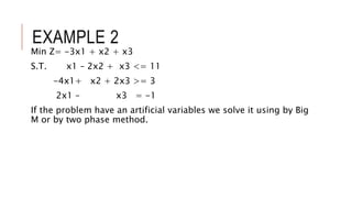
Write the problem in canonical form [using big M]
Min Z= -3x1 + x2 + x3 + Mx6 + Mx7
S.T. x1 – 2x2 + x3 + x4 = 11
-4x1 + x2 +2x3 – x5 + x6 = 3
-2x1 + x3 + x7 = 1

17. EXAMPLE 2
Iteration 1: Basic: x4=11, x6=3, x7=1.
Z=Mx6+Mx7=3M+M=4M, B=Id.
CB Basic B-1 b Enteri
ng
Pivot
0 X4 1 0 0 11
M X6 0 1 0 3
M X7 0 0 1 1

18. EXAMPLE 2
MMMPCC
MMMPCC
MMMPCC
MMMPCC
MMBCB




























 














 
0
1
0
).,,0(0
31
1
2
1
).,,0(1
1
0
1
2
).,,0(1
36
2
4
1
).,,0(3
),,0(
555
333
222
111
1






19. EXAMPLE 2
X3 is entering
P3new= B-1*P3old = , b=
X3=min{11,3/2,1}=1, so X7 is leaving
The pivot column must be transform to , X7 Place
We do the same operations to B-1 and we got
b= B-1 * bold
= =
1
2
1
11
3
1
0
0
1
1
2
1
-2R3+R2-
>R2
-R3+R1->R1
0
0
1 1 0 -1
0 1 -2
0 0 1
1 0 -1
0 1 -2
0 0 1
11
3
1
10
1
1

20. EXAMPLE 2
Iteration 2: Basic: x4=11-1=10, x6=3-2=1, x3=1. Z=1+M
CB Basic B-1 b Enteri
ng
Pivot
0 X4 1 0 -1 10
M X6 0 1 -2 1
1 X3 0 0 1 1

21. EXAMPLE 2
MMMPCC
MMMPCC
MMPCC
MMMBCB


















 

























 
0
1
0
).12,,0(0
1
0
1
2
).12,,0(1
1
2
4
1
).12,,0(3
)12,,0(
100
2-10
1-01
)1,,0(
555
222
111
1





22. EXAMPLE 2
X2 is entering
P2new= B-1*P2old = =
X2=min{-5,1,Inf.}=1, so X6 is leaving
The pivot column must be transform to , X6 Place
We do the same operations to B-1 and we got
b= B-1 * bold
= =
-2
1
0
0
1
0
-2
1
0
2R1+R1->R1
0
1
0 1 2 -5
0 1 -2
0 0 1
1 2 -5
0 1 -2
0 0 1
11
3
1
12
1
1
1 0 -1
0 1 -2
0 0 1
-2
1
0

23. EXAMPLE 2
Iteration 2: Basic: x4=11-1=10, x6=3-2=1, x3=1. Z=1+M
CB Basic B-1 b Enteri
ng
Pivot
0 X4 1 2 -5 10
1 X2 0 1 -2 1
1 X3 0 0 1 1

24. EXAMPLE 2
1
0
1
0
).1,1,0(0
1
2
4
1
).1,1,0(3
)1,1,0(
100
2-10
5-21
)1,1,0(
555
111
1


































 
PCC
PCC
BCB




25. EXAMPLE 2
X1 is entering
P1new= B-1*P1old = =
X1=min{4,inf.,-1/2}=1, so X4 is leaving
The pivot column must be transform to , X4 Place
We do the same operations to B-1 and we got
b= B-1 * bold
= =
1
-4
-2
1
0
0
3
0
-2
1/3R1->R1
2R1+R3 -
>R3
1
0
0
1/3 2/3 -
5/3
0 1 -2
2/3 4/3 -
7/3
11
3
1
4
1
9
1 2 -5
0 1 -2
0 0 1
3
0
-2
1/3 2/3 -
5/3
0 1 -2
2/3 4/3 -
7/3

26. EXAMPLE 2
Iteration 2: Basic: x4=11-1=10, x6=3-2=1, x3=1. Z=1+M
CB Basic B-1 b Enteri
ng
Pivot
-3 X1 1/3 2/3 -5/3 4
1 X2 0 1 -2 1
1 X3 2/3 4/3 -7/3 9

27. EXAMPLE 2
-2Z9,x31,x24,x1:issolutionoptimalThe
variableenteringNo
3/1
)3/2,3/1,3/1(
5
1


 
C
BCB

28. EXAMPLE 3
Min Z= 5x1 + 2x2
S.T. -x1 + 2x2 + x3 = 4
3x1 + 2x2 + x4 = 14
x1 – x2 + x5 = 3

29. EXAMPLE 3
Iteration 1: Basic: x3=4, x4=14, x5=3. Z=0.
CB Basic B-1 b Enteri
ng
Pivot
0 X3 1 0 0 4
0 X4 0 1 0 14
0 X5 0 0 1 3

30. EXAMPLE 3
leavingisx5
33,3}min{-4,14/toequalitsandenteringisx1
2
55
)0,0,0(
222
111
1



 
PCC
PCC
BCB




31. EXAMPLE 2
P1new= B-1*P1old = =
The pivot column must be transform to
We do the same operations to B-1 and we got
b= B-1 * bold
= =
-1
3
1
0
0
1
-1
3
1
R3+R1->R1
-3R3+R2 -
>R2
0
0
1
1 0 1
0 1 -3
0 0 1
1 0 0
0 1 0
0 0 1
-1
3
1
4
14
3
1 0 1
0 1 -3
0 0 1
7
5
3

32. EXAMPLE 3
Iteration 2: Basic: x3=4, x4=14, x1=3. Z=5.
CB Basic B-1 b Enteri
ng
Pivot
0 X3 1 0 1 7
0 X4 0 1 -3 5
0 X1 0 0 1 3

33. EXAMPLE 3
leavingisx4
1}min{7,1,-3toequalitsandenteringisx2
5
1
2
2
)3,0,0(2
)3,0,0(
100
3-10
101
)3,0,0(
222
1

























 
PCC
BCB



34. EXAMPLE 2
P2new= B-1*P2old = =
The pivot column must be transform to
We do the same operations to B-1 and we got
2
2
-1
0
1
0
1
5
-1
1/5R2->R2
-R2+R1->R1
R2+R3 ->R3
0
1
0
1 0 1
0 1 -3
0 0 1
1
5
-1
1 -1/5
8/5
0 1/5 -
3/5
0 1/5
2/5

35. EXAMPLE 3
Iteration 3: Basic: x3=7, x2=5, x5=3. Z=11.
This is the optimal solution because there is no entering
variables.
CB Basic B-1 b Enteri
ng
Pivot
0 X3 1 -1/5 8/5
0 X2 0 1/5 -3/5
0 X1 0 1/5 2/5