The document discusses a blog that provides free solutions manuals and solved exercises for many university textbooks. It states that the solutions manuals contain clear explanations of all the exercises from the textbooks. It invites the reader to visit the blog to download the solutions manuals for free.


![]
[CO
]
][HCO
[H
2
3
1
−
+
=
K (1)
]
[HCO
]
][CO
[H
3
2
3
2 −
−
+
=
K (2)
]
][OH
[H
= + −
w
K (3)
]
[CO
]
[HCO
]
[CO
= 2
3
3
2
−
−
+
+
T
c (4)
]
[H
]
[OH
+
]
[CO
2
]
[HCO
=
Alk +
2
3
3 −
+ −
−
−
(5)
One way is to combine the equations to produce a single polynomial. Equations 1 and 2 can be solved
for
1
3
3
2
]
][HCO
[H
]
CO
[H *
K
−
+
=
]
[HCO
]
[H
]
[CO
3
2
2
3 −
+
−
=
K
These results can be substituted into Eq. 4, which can be solved for
T
c
F0
3
2 ]
CO
[H *
= T
c
F1
3 ]
[HCO =
−
T
c
F2
2
3 ]
[CO =
−
where F0, F1, and F2 are the fractions of the total inorganic carbon in carbon dioxide, bicarbonate and
carbonate, respectively, where
2
1
1
2
2
0
]
[H
]
[H
]
[H
=
K
K
K
F
+
+ +
+
+
2
1
1
2
1
1
]
[H
]
[H
]
[H
=
K
K
K
K
F
+
+ +
+
+
2
1
1
2
2
1
2
]
[H
]
[H
=
K
K
K
K
K
F
+
+ +
+
Now these equations, along with the Eq. 3 can be substituted into Eq. 5 to give
Alk
]
[H
]
[H
+
2
=
0 +
+
2
1 −
−
+ w
T
T K
c
F
c
F
Although it might not be apparent, this result is a fourth-order polynomial in [H+].
( ) ( ) 2
+
1
1
2
1
3
+
1
4
+
]
H
[
Alk
]
H
[
Alk
]
H
[ T
w c
K
K
K
K
K
K −
−
+
+
+
+
( ) 0
]
H
[
2
Alk 2
1
+
2
1
1
2
1 =
−
−
−
+ w
T
w K
K
K
c
K
K
K
K
K
K
Substituting parameter values gives
0
10
512
.
2
]
H
[
10
055
.
1
]
H
[
10
012
.
5
]
H
[
10
001
.
2
]
H
[ 31
+
19
2
+
10
3
+
3
4
+
=
×
−
×
−
×
−
×
+ −
−
−
−
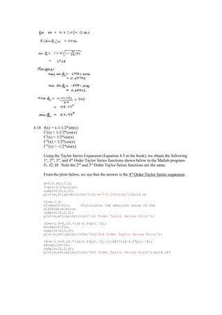
This equation can be solved for [H+] = 2.51x10⁻⁷ (pH = 6.6). This value can then be used to compute
8
7
14
10
98
.
3
10
51
.
2
10
]
[OH −
−
−
−
×
=
×
=](https://image.slidesharecdn.com/solucionariodechapraycanalequintae-230530034223-b54cf15a/85/Solucionario_de_Chapra_y_Canale_Quinta_E-pdf-28-320.jpg)
![( )
( ) ( )
( ) 001
.
0
10
3
33304
.
0
10
3
10
10
10
2.51
10
10
2.51
10
2.51
=
]
CO
H
[ 3
3
3
.
10
3
.
6
7
-
3
.
6
2
7
-
2
7
-
3
2
*
=
×
=
×
+
×
+
×
× −
−
−
−
−
( )
( ) ( )
( ) 002
.
0
10
3
666562
.
0
10
3
10
10
10
2.51
10
10
2.51
10
2.51
10
=
]
HCO
[ 3
3
3
.
10
3
.
6
7
-
3
.
6
2
7
-
-7
3
.
6
3 =
×
=
×
+
×
+
×
× −
−
−
−
−
−
−
( ) ( )
( ) M
4
3
3
3
.
10
3
.
6
7
-
3
.
6
2
7
-
3
.
10
3
.
6
2
3 10
33
.
1
10
3
000133
.
0
10
3
10
10
10
2.51
10
10
2.51
10
10
=
]
CO
[ −
−
−
−
−
−
−
−
−
×
=
×
=
×
+
×
+
×
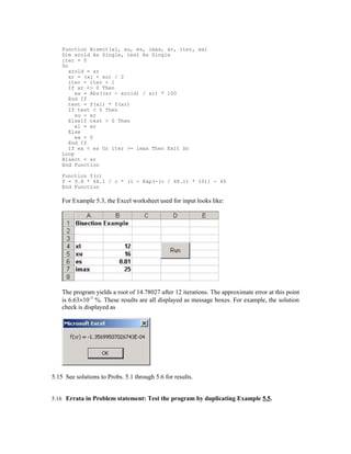
8.14 The integral can be evaluated as
−
+
−
=
+
− ∫ in
out
in
out
max
max
max
ln
1
1
out
in
C
C
C
C
K
k
dc
k
C
k
K
C
C
Therefore, the problem amounts to finding the root of
−
+
+
= in
out
in
out
max
out ln
1
)
( C
C
C
C
K
k
F
V
C
f
Excel solver can be used to find the root:](https://image.slidesharecdn.com/solucionariodechapraycanalequintae-230530034223-b54cf15a/85/Solucionario_de_Chapra_y_Canale_Quinta_E-pdf-29-320.jpg)


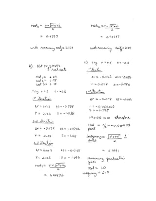
![8.24
%Region from x=8 to x=10
x1=[8:.1:10];
y1=20*(x1-(x1-5))-15-57;
figure (1)
plot(x1,y1)
grid
%Region from x=7 to x=8
x2=[7:.1:8];
y2=20*(x2-(x2-5))-57;
figure (2)
plot(x2,y2)
grid
%Region from x=5 to x=7
x3=[5:.1:7];
y3=20*(x3-(x3-5))-57;
figure (3)
plot(x3,y3)
grid
%Region from x=0 to x=5
x4=[0:.1:5];
y4=20*x4-57;
figure (4)
plot(x4,y4)
grid
%Region from x=0 to x=10
figure (5)
plot(x1,y1,x2,y2,x3,y3,x4,y4)
grid
title('shear diagram')
a=[20 -57]
roots(a)
a =
20 -57
ans =
2.8500
0 1 2 3 4 5 6 7 8 9 10
-60
-40
-20
0
20
40
60
s hear diagram](https://image.slidesharecdn.com/solucionariodechapraycanalequintae-230530034223-b54cf15a/85/Solucionario_de_Chapra_y_Canale_Quinta_E-pdf-33-320.jpg)
![8.25
%Region from x=7 to x=8
x2=[7:.1:8];
y2=-10*(x2.^2-(x2-5).^2)+150+57*x2;
figure (2)
plot(x2,y2)
grid
%Region from x=5 to x=7
x3=[5:.1:7];
y3=-10*(x3.^2-(x3-5).^2)+57*x3;
figure (3)
plot(x3,y3)
grid
%Region from x=0 to x=5
x4=[0:.1:5];
y4=-10*(x4.^2)+57*x4;
figure (4)
plot(x4,y4)
grid
%Region from x=0 to x=10
figure (5)
plot(x1,y1,x2,y2,x3,y3,x4,y4)
grid
title('moment diagram')
a=[-43 250]
roots(a)
a =
-43 250
ans =
5.8140
0 1 2 3 4 5 6 7 8 9 10
-60
-40
-20
0
20
40
60
80
100
m om ent diagram](https://image.slidesharecdn.com/solucionariodechapraycanalequintae-230530034223-b54cf15a/85/Solucionario_de_Chapra_y_Canale_Quinta_E-pdf-34-320.jpg)
![8.26 A Matlab script can be used to determine that the slope equals zero at x = 3.94 m.
%Region from x=8 to x=10
x1=[8:.1:10];
y1=((-10/3)*(x1.^3-(x1-5).^3))+7.5*(x1-8).^2+150*(x1-7)+(57/2)*x1.^2-
238.25;
figure (1)
plot(x1,y1)
grid
%Region from x=7 to x=8
x2=[7:.1:8];
y2=((-10/3)*(x2.^3-(x2-5).^3))+150*(x2-7)+(57/2)*x2.^2-238.25;
figure (2)
plot(x2,y2)
grid
%Region from x=5 to x=7
x3=[5:.1:7];
y3=((-10/3)*(x3.^3-(x3-5).^3))+(57/2)*x3.^2-238.25;
figure (3)
plot(x3,y3)
grid
%Region from x=0 to x=5
x4=[0:.1:5];
y4=((-10/3)*(x4.^3))+(57/2)*x4.^2-238.25;
figure (4)
plot(x4,y4)
grid
%Region from x=0 to x=10
figure (5)
plot(x1,y1,x2,y2,x3,y3,x4,y4)
grid
title('slope diagram')
a=[-10/3 57/2 0 -238.25]
roots(a)
a =
-3.3333 28.5000 0 -238.2500
ans =
7.1531
3.9357
-2.5388
0 1 2 3 4 5 6 7 8 9 10
-250
-200
-150
-100
-50
0
50
100
150
200
slope diagram
8.27](https://image.slidesharecdn.com/solucionariodechapraycanalequintae-230530034223-b54cf15a/85/Solucionario_de_Chapra_y_Canale_Quinta_E-pdf-35-320.jpg)
![%Region from x=8 to x=10
x1=[8:.1:10];
y1=(-5/6)*(x1.^4-(x1-5).^4)+(15/6)*(x1-8).^3+75*(x1-7).^2+(57/6)*x1.^3-
238.25*x1;
figure (1)
plot(x1,y1)
grid
%Region from x=7 to x=8
x2=[7:.1:8];
y2=(-5/6)*(x2.^4-(x2-5).^4)+75*(x2-7).^2+(57/6)*x2.^3-238.25*x2;
figure (2)
plot(x2,y2)
grid
%Region from x=5 to x=7
x3=[5:.1:7];
y3=(-5/6)*(x3.^4-(x3-5).^4)+(57/6)*x3.^3-238.25*x3;
figure (3)
plot(x3,y3)
grid
%Region from x=0 to x=5
x4=[0:.1:5];
y4=(-5/6)*(x4.^4)+(57/6)*x4.^3-238.25*x4;
figure (4)
plot(x4,y4)
grid
%Region from x=0 to x=10
figure (5)
plot(x1,y1,x2,y2,x3,y3,x4,y4)
grid
title('displacement curve')
a =
-3.3333 28.5000 0 -238.2500
ans =
7.1531
3.9357
-2.5388
Therefore, other than the end supports, there are no points of zero displacement along the beam.
0 1 2 3 4 5 6 7 8 9 10
-600
-500
-400
-300
-200
-100
0
dis plac em ent c urve](https://image.slidesharecdn.com/solucionariodechapraycanalequintae-230530034223-b54cf15a/85/Solucionario_de_Chapra_y_Canale_Quinta_E-pdf-36-320.jpg)


![0
20
40
60
80
100
120
1 2 3
8.44
% Shuttle Liftoff Engine Angle
% Newton-Raphson Method of iteratively finding a single root
format long
% Constants
LGB = 4.0; LGS = 24.0; LTS = 38.0;
WS = 0.230E6; WB = 1.663E6;
TB = 5.3E6; TS = 1.125E6;
es = 0.5E-7; nmax = 200;
% Initial estimate in radians
x = 0.25
%Calculation loop
for i=1:nmax
fx = LGB*WB-LGB*TB-LGS*WS+LGS*TS*cos(x)-LTS*TS*sin(x);
dfx = -LGS*TS*sin(x)-LTS*TS*cos(x);
xn=x-fx/dfx;
%convergence check
ea=abs((xn-x)/xn);
if (ea<=es)
fprintf('convergence: Root = %f radians n',xn)
theta = (180/pi)*x;
fprintf('Engine Angle = %f degrees n',theta)
break
end
x=xn;
x
end
% Shuttle Liftoff Engine Angle
% Newton-Raphson Method of iteratively finding a single root
% Plot of Resultant Moment vs Engine Anale
format long
% Constants
LGB = 4.0; LGS = 24.0; LTS = 38.0;
WS = 0.195E6; WB = 1.663E6;
TB = 5.3E6; TS = 1.125E6;
x=-5:0.1:5;
fx = LGB*WB-LGB*TB-LGS*WS+LGS*TS*cos(x)-LTS*TS*sin(x);
plot(x,fx)
grid
axis([-6 6 -8e7 4e7])
title('Space Shuttle Resultant Moment vs Engine Angle')
xlabel('Engine angle ~ radians')
ylabel('Resultant Moment ~ lb-ft')
x =
0.25000000000000
x =
0.15678173034564
x =
0.15518504730788
x =
0.15518449747125](https://image.slidesharecdn.com/solucionariodechapraycanalequintae-230530034223-b54cf15a/85/Solucionario_de_Chapra_y_Canale_Quinta_E-pdf-44-320.jpg)


1
.
3
2
9
sech
'
9
tanh
2
2
2
=
−
=
−
=
o
x
x
x
x
f
x
x
f
( )
( )
x
f
x
f
x
x i
i '
1 −
=
+
iteration xi+1
1 2.9753
2 3.2267
3 2.5774
4 7.9865
The solution diverges from its real root of x = 3. Due to the concavity of the slope, the next iteration
will always diverge. The sketch should resemble figure 6.6(a).
6.23
SOLUTION:](https://image.slidesharecdn.com/solucionariodechapraycanalequintae-230530034223-b54cf15a/85/Solucionario_de_Chapra_y_Canale_Quinta_E-pdf-83-320.jpg)


![>> roots (d)
with the expected result that the remaining roots of the original polynomial are found
ans =
8.0000
-4.0000
1.0000
We can now multiply d by b to come up with the original polynomial,
>> conv(d,b)
ans =
1 -9 -20 204 208 -384
Finally, we can determine all the roots of the original polynomial by
>> r=roots(a)
r =
8.0000
6.0000
-4.0000
-2.0000
1.0000
7.15
p=[0.7 -4 6.2 -2];
roots(p)
ans =
3.2786
2.0000
0.4357
p=[-3.704 16.3 -21.97 9.34];
roots(p)
ans =
2.2947
1.1525
0.9535
p=[1 -2 6 -2 5];
roots(p)
ans =
1.0000 + 2.0000i
1.0000 - 2.0000i
-0.0000 + 1.0000i
-0.0000 - 1.0000i
7.16 Here is a program written in Compaq Visual Fortran 90,
PROGRAM Root
Use IMSL !This establishes the link to the IMSL libraries](https://image.slidesharecdn.com/solucionariodechapraycanalequintae-230530034223-b54cf15a/85/Solucionario_de_Chapra_y_Canale_Quinta_E-pdf-95-320.jpg)

![7.18
I) Graphically:
EDU»C=[1 3.6 0 -36.4];roots(C)
ans = -3.0262+ 2.3843i
-3.0262- 2.3843i
2.4524
The answer is 2.4524 considering it is the only real root.
II) Using the Roots Function:
EDU» x=-1:0.001:2.5;f=x.^3+3.6.*x.^2-36.4;plot(x,f);grid;zoom
By zooming in the plot at the desired location, we get the same answer of 2.4524.
2.4523 2.45232.4524 2.4524 2.4524 2.4524 2.45242.4524 2.4524 2.4524 2.4524
-6
-4
-2
0
2
4
x 10
-4
7.19
Excel Solver Solution: The 3 functions can be set up as roots problems:
0
2
)
,
,
(
0
2
)
,
,
(
0
3
)
,
,
(
2
3
2
2
2
2
1
=
−
−
=
=
−
+
=
=
+
−
=
u
a
a
v
u
a
f
v
u
v
u
a
f
v
u
a
v
u
a
f](https://image.slidesharecdn.com/solucionariodechapraycanalequintae-230530034223-b54cf15a/85/Solucionario_de_Chapra_y_Canale_Quinta_E-pdf-97-320.jpg)


![9.14
Here is a VBA program to implement matrix multiplication and solve Prob. 9.3 for the case
of [X]×[Y].
Option Explicit
Sub Mult()
Dim i As Integer, j As Integer
Dim l As Integer, m As Integer, n As Integer
Dim x(10, 10) As Single, y(10, 10) As Single
Dim w(10, 10) As Single
l = 2
m = 2
n = 3
x(1, 1) = 1: x(1, 2) = 6
x(2, 1) = 3: x(2, 2) = 10
x(3, 1) = 7: x(3, 2) = 4
y(1, 1) = 6: y(2, 1) = 0
y(2, 1) = 1: y(2, 2) = 4
Call Mmult(x(), y(), w(), m, n, l)
For i = 1 To n
For j = 1 To l
MsgBox w(i, j)
Next j
Next i
End Sub
Sub Mmult(y, z, x, n, m, p)
Dim i As Integer, j As Integer, k As Integer
Dim sum As Single
For i = 1 To m
For j = 1 To p
sum = 0
For k = 1 To n
sum = sum + y(i, k) * z(k, j)
Next k
x(i, j) = sum
Next j
Next i
End Sub
9.15
Here is a VBA program to implement the matrix transpose and solve Prob. 9.3 for the case of
[X]T
.
Option Explicit
Sub Mult()
Dim i As Integer, j As Integer
Dim m As Integer, n As Integer
Dim x(10, 10) As Single, y(10, 10) As Single
n = 3
m = 2
x(1, 1) = 1: x(1, 2) = 6
x(2, 1) = 3: x(2, 2) = 10](https://image.slidesharecdn.com/solucionariodechapraycanalequintae-230530034223-b54cf15a/85/Solucionario_de_Chapra_y_Canale_Quinta_E-pdf-104-320.jpg)


![10.17
( )
3
10
3
2
)
2
(
6
3
2
0
)
1
(
3
2
4
0
=
+
⇒
=
⋅
−
=
−
⇒
=
⋅
=
+
−
⇒
=
⋅
c
b
C
B
c
a
C
A
b
a
B
A
Solve the three equations using Matlab:
>> A=[-4 2 0; 2 0 –3; 0 3 1]
b=[3; -6; 10]
x=inv(A)*b
x = 0.525
2.550
2.350
Therefore, a = 0.525, b = 2.550, and c = 2.350.
10.18
k
b
a
j
c
a
i
c
b
c
k
b
a
j
i
B
A
)
2
(
)
2
4
(
)
4
(
4
1
2
)
( +
+
+
−
−
−
−
=
−
−
=
×
k
b
a
j
c
a
i
c
b
c
k
b
a
j
i
C
A
)
3
(
)
2
(
)
3
2
(
2
3
1
)
( +
+
−
−
−
=
=
×
k
b
a
j
c
a
i
c
b
C
A
B
A
)
4
(
)
2
(
)
4
2
(
)
(
)
( +
+
+
−
−
−
−
=
×
+
×](https://image.slidesharecdn.com/solucionariodechapraycanalequintae-230530034223-b54cf15a/85/Solucionario_de_Chapra_y_Canale_Quinta_E-pdf-116-320.jpg)
![Therefore,
k
c
j
b
i
a
r
b
a
j
c
a
i
c
b
)
1
4
(
)
2
3
(
)
6
5
(
)
4
(
)
2
(
)
4
2
( +
−
+
−
+
+
=
+
+
−
−
+
−
−
We get the following set of equations ⇒
6
4
2
5
6
5
4
2 =
−
−
−
⇒
+
=
−
− c
b
a
a
c
b (1)
2
3
2
2
3
2 −
=
−
−
⇒
−
=
− c
b
a
b
c
a (2)
1
4
4
1
4
4 =
−
+
⇒
+
−
=
+ c
b
a
c
b
a (3)
In Matlab:
A=[-5 -5 -4 ; 2 -3 -1 ; 4 1 -4]
B=[ 6 ; -2 ; 1] ; x = inv (A) * b
Answer ⇒ x = -3.6522
-3.3478
4.7391
a = -3.6522, b = -3.3478, c = 4.7391
10.19
(I) 1
1
)
0
(
1
)
0
( =
⇒
=
+
⇒
= b
b
a
f
1
2
1
)
2
(
1
)
2
( =
+
⇒
=
+
⇒
= d
c
d
c
f
(II) If f is continuous, then at x = 1
0
)
1
(
)
1
( =
−
−
+
⇒
+
=
+
⇒
+
=
+ d
c
b
a
d
c
b
a
d
cx
b
ax
(III) 4
=
+ b
a
=
−
−
4
0
1
1
0
0
1
1
1
1
1
1
2
2
0
0
0
0
1
0
d
c
b
a
Solve using Matlab ⇒
10.20 MATLAB provides a handy way to solve this problem.
a = 3
b = 1
c = -3
d = 7](https://image.slidesharecdn.com/solucionariodechapraycanalequintae-230530034223-b54cf15a/85/Solucionario_de_Chapra_y_Canale_Quinta_E-pdf-117-320.jpg)
![(a)
>> a=hilb(3)
a =
1.0000 0.5000 0.3333
0.5000 0.3333 0.2500
0.3333 0.2500 0.2000
>> b=[1 1 1]'
b =
1
1
1
>> c=a*b
c =
1.8333
1.0833
0.7833
>> format long e
>> x=ab
>> x =
9.999999999999991e-001
1.000000000000007e+000
9.999999999999926e-001
(b)
>> a=hilb(7);
>> b=[1 1 1 1 1 1 1]';
>> c=a*b;
>> x=ab
x =
9.999999999914417e-001
1.000000000344746e+000
9.999999966568566e-001
1.000000013060454e+000
9.999999759661609e-001
1.000000020830062e+000
9.999999931438059e-001
(c)
>> a=hilb(10);
>> b=[1 1 1 1 1 1 1 1 1 1]';
>> c=a*b;
>> x=ab
x =
9.999999987546324e-001
1.000000107466305e+000
9.999977129981819e-001
1.000020777695979e+000
9.999009454847158e-001
1.000272183037448e+000
9.995535966572223e-001
1.000431255894815e+000
9.997736605804316e-001
1.000049762292970e+000](https://image.slidesharecdn.com/solucionariodechapraycanalequintae-230530034223-b54cf15a/85/Solucionario_de_Chapra_y_Canale_Quinta_E-pdf-118-320.jpg)


![Matlab solution to Prob. 11.11 (ii):
a=[1 4 9 16;4 9 16 25;9 16 25 36;16 25 36 49]
a =
1 4 9 16
4 9 16 25
9 16 25 36
16 25 36 49
b=[30 54 86 126]
b =
30 54 86 126
b=b'
b =
30
54
86
126
x=ab
Warning: Matrix is close to singular or badly scaled.
Results may be inaccurate. RCOND = 2.092682e-018.
x =
1.1053
0.6842
1.3158
0.8947
x=inv(a)*b
Warning: Matrix is close to singular or badly scaled.
Results may be inaccurate. RCOND = 2.092682e-018.
x =
0
0
0
0
cond(a)
ans =
4.0221e+017](https://image.slidesharecdn.com/solucionariodechapraycanalequintae-230530034223-b54cf15a/85/Solucionario_de_Chapra_y_Canale_Quinta_E-pdf-123-320.jpg)


![12.10 Mass balances can be written for each reactor as
1
,
1
1
1
,
in
in
,
in
0 A
A
A c
V
k
c
Q
c
Q −
−
=
1
,
1
1
1
,
in
0 A
B c
V
k
c
Q +
=
2
,
2
2
2
,
32
in
3
,
32
1
,
in )
(
0 A
A
A
A c
V
k
c
Q
Q
c
Q
c
Q −
+
−
+
=
2
,
2
2
2
,
32
in
3
,
32
1
,
in )
(
0 A
B
B
B c
V
k
c
Q
Q
c
Q
c
Q +
+
−
+
=
3
,
3
3
3
,
43
in
4
,
43
2
,
32
in )
(
)
(
0 A
A
A
A c
V
k
c
Q
Q
c
Q
c
Q
Q −
+
−
+
+
=
3
,
3
3
3
,
43
in
4
,
43
2
,
32
in )
(
)
(
0 A
B
B
B c
V
k
c
Q
Q
c
Q
c
Q
Q +
+
−
+
+
=
4
,
4
4
4
,
43
in
3
,
43
in )
(
)
(
0 A
A
A c
V
k
c
Q
Q
c
Q
Q −
+
−
+
=
4
,
4
4
4
,
43
in
3
,
43
in )
(
)
(
0 A
B
B c
V
k
c
Q
Q
c
Q
Q +
+
−
+
=
Collecting terms, the system can be expresses in matrix form as
[A]{C} = {B}
where
[A] =
−
−
−
−
−
−
−
−
−
−
−
−
−
−
13
5
.
2
13
0
0
0
0
0
0
5
.
15
0
13
0
0
0
0
3
0
18
50
15
0
0
0
0
3
0
68
0
15
0
0
0
0
5
0
15
5
.
7
10
0
0
0
0
5
0
5
.
22
0
10
0
0
0
0
0
0
10
25
.
1
0
0
0
0
0
0
0
25
.
11
[B]T
= [10 0 0 0 0 0 0 0 0 0] [C]T
= [cA,1 cB,1 cA,2 cB,2 cA,3 cB,3 cA,4 cB,4]
The system can be solved for [C]T
= [0.889 0.111 0.416 0.584 0.095 0.905 0.080
0.920].
A
B
0
0.2
0.4
0.6
0.8
1
0 1 2 3 4
12.11 Assuming a unit flow for Q1, the simultaneous equations can be written in matrix form
as](https://image.slidesharecdn.com/solucionariodechapraycanalequintae-230530034223-b54cf15a/85/Solucionario_de_Chapra_y_Canale_Quinta_E-pdf-132-320.jpg)
![
=
−
−
−
−
−
−
−
0
0
1
0
0
0
1
1
1
0
0
0
0
0
1
1
1
0
0
0
0
0
1
1
3
1
0
0
0
0
0
1
2
1
0
0
0
0
0
1
2
1
7
6
5
4
3
2
Q
Q
Q
Q
Q
Q
These equations can be solved to give [Q]T
= [0.7321 0.2679 0.1964 0.0714 0.0536
0.0178].](https://image.slidesharecdn.com/solucionariodechapraycanalequintae-230530034223-b54cf15a/85/Solucionario_de_Chapra_y_Canale_Quinta_E-pdf-133-320.jpg)


![0
872
.
0
744
.
1
100
744
.
1
872
.
0
=
−
+
−
=
−
+
−
B
A
B
A
Plug into equations 9.10 and 9.11:
N
a
a
a
a
b
a
b
a
x
N
a
a
a
a
b
a
b
a
x
87
.
45
80192
.
3
4
.
174
94
.
22
80192
.
3
2
.
87
21
12
22
11
1
21
2
11
2
21
12
22
11
2
12
1
22
1
=
=
−
−
=
=
=
−
−
=
12.21
k
j
i
k
j
i
T ˆ
549
.
0
ˆ
824
.
0
ˆ
1374
.
0
4
6
1
ˆ
4
ˆ
6
ˆ
1
2
2
2
−
+
=
+
+
−
+
0
)
1
(
549
.
0
)
1
(
5 =
−
+
−
=
∑ T
M y
kN
T 107
.
9
=
kN
T
kN
T
kN
T z
y
x 5
,
50
.
7
,
251
.
1 −
=
=
=
∴
0
)
3
(
)
3
(
5
)
4
(
5
.
7
)
3
(
5 =
+
−
+
−
+
−
=
∑ z
x B
M kN
Bz 20
=
0
)
3
(
)
3
(
251
.
1
)
3
(
5
.
7 =
+
+
=
∑ x
z B
M
kN
Bx 751
.
3
−
=
0
20
5
5 =
+
+
−
+
−
=
∑ z
z A
F
kN
Az 10
−
=
0
251
.
1
751
.
3 =
+
−
+
=
∑ x
x A
F kN
Ax 5
.
2
=
0
50
.
7 =
+
=
∑ y
y A
F kN
Ay 5
.
7
−
=
12.22 This problem was solved using Matlab.
A = [1 0 0 0 0 0 0 0 1 0
0 0 1 0 0 0 0 1 0 0
0 1 0 3/5 0 0 0 0 0 0
-1 0 0 -4/5 0 0 0 0 0 0
0 -1 0 0 0 0 3/5 0 0 0
0 0 0 0 -1 0 -4/5 0 0 0
0 0 -1 -3/5 0 1 0 0 0 0
0 0 0 4/5 1 0 0 0 0 0
0 0 0 0 0 -1 -3/5 0 0 0
0 0 0 0 0 0 4/5 0 0 1];
b = [0 0 –54 0 0 24 0 0 0 0];
x=inv(A)*b
x =](https://image.slidesharecdn.com/solucionariodechapraycanalequintae-230530034223-b54cf15a/85/Solucionario_de_Chapra_y_Canale_Quinta_E-pdf-140-320.jpg)


![12.27 This problem can be solved directly on a calculator capable of doing matrix operations
or on Matlab.
a=[60 -40 0
-40 150 -100
0 -100 130];
b=[200
0
230];
x=inv(a)*b
x =
7.7901
6.6851
6.9116
Therefore,
I1 = 7.79 A
I2 = 6.69 A
I3 = 6.91 A
12.28 This problem can be solved directly on a calculator capable of doing matrix operations
or on Matlab.
a=[17 -8 -3](https://image.slidesharecdn.com/solucionariodechapraycanalequintae-230530034223-b54cf15a/85/Solucionario_de_Chapra_y_Canale_Quinta_E-pdf-144-320.jpg)
![-2 6 -3
-1 -4 13];
b=[480
0
0];
x=inv(a)*b
x =
37.3585
16.4151
7.9245
Therefore,
V1 = 37.4 V
V2 = 16.42 V
V3 = 7.92 V
12.29 This problem can be solved directly on a calculator capable of doing matrix operations
or on Matlab.
a=[6 0 -4 1
0 8 -8 -1
-4 -8 18 0
-1 1 0 0];
b=[0
-20
0
10];
x=inv(a)*b
x =
-7.7778
2.2222
-0.7407
43.7037
Therefore,
I1 = -7.77 A
I2 = 2.22 A
I3 = -.741 A
Vs = 43.7 V
12.30 This problem can be solved directly on a calculator capable of doing matrix operations
or on Matlab.
a=[55 0 -25
0 37 -4
-25 -4 29];
b=[-200
-250
100];
x=inv(a)*b](https://image.slidesharecdn.com/solucionariodechapraycanalequintae-230530034223-b54cf15a/85/Solucionario_de_Chapra_y_Canale_Quinta_E-pdf-145-320.jpg)


![k1=10;
k2=40;
k3=40;
k4=10;
m1=1;
m2=1;
m3=1;
km=[(1/m1)*(k2+k1), -(k2/m1),0; -(k2/m2), (1/m2)*(k2+k3), -(k3/m2);
0, -(k3/m3),(1/m3)*(k3+k4)];
X=[0.05;0.04;0.03];
kmx=km*X
kmx =
0.9000
0.0000
-0.1000
Therefore, 1
x
= -0.9, 2
x
= 0 , and 3
x
= 0.1 m/s2
.](https://image.slidesharecdn.com/solucionariodechapraycanalequintae-230530034223-b54cf15a/85/Solucionario_de_Chapra_y_Canale_Quinta_E-pdf-149-320.jpg)


![1 X Y Z Total Constraint
2 Amount 0 0 0
3 Performance 1 1 1 0 6
4 Safety 1 1 0 0 3
5 X-Y 1 -1 0 0 0
6 Z-Y 0 -0.5 1 0 0
7 Cost 0.15 0.025 0.05 0
A B C D E F G
1 Z1 Z2 Z3 W total constraint
2 amount 4000 3500 0 500
3 amount X 1 1 0 0 7500 7500
4 amount Y 2.5 0 1 0 10000 10000
5 amount W 1 -1 -1 -1 0 0
6 profit 2500 -50 200 -300 9675000
Set target cell: F6
Equal to ● max ❍ min ❍ value of 0
By changing cells
B2:E2
Subject to constraints:
B2≥0
C2≥0
F3≤G3
F4≤G4
F5=G5
A B C D E F G
1 Z1 Z2 Z3 W total constraint
2 amount 0 0 0 0
3 amount X 1 1 0 0 0 7500
4 amount Y 2.5 0 1 0 0 10000
5 amount W 1 -1 -1 -1 0 0
6 profit 2500 -50 200 -300 0
Microsoft Excel 5.0c Sensitivity Report
Worksheet: [PROB1605.XLS]Sheet3
Report Created: 12/12/97 9:47
Changing Cells
Final Reduced Objective Allowable Allowable
Cell Name Value Cost Coefficient Increase Decrease
$B$2 amount Product 1 150 0 30 0.833333333 2.5
$C$2 amount Product 2 125 0 30 1.666666667 1
$D$2 amount Product 3 175 0 35 35 5
Constraints
Final Shadow Constraint Allowable Allowable
Cell Name Value Price R.H. Side Increase Decrease
$E$3 material total 3000 0.625 3000 1E+30 1E+30
$E$4 time total 55 12.5 55 1E+30 1E+30
$E$5 storage total 450 26.25 450 1E+30 1E+30
A B C D E F
1 Product 1 Product 2 Product 3 total constraint
2 amount 150 125 175
3 material 5 4 10 3000 3000](https://image.slidesharecdn.com/solucionariodechapraycanalequintae-230530034223-b54cf15a/85/Solucionario_de_Chapra_y_Canale_Quinta_E-pdf-167-320.jpg)


![20.11 The best fit equation can be determined by nonlinear regression as
]
[
8766
.
0
]
[
84
.
98
]
[
F
F
B
+
=
0
20
40
60
80
100
120
0 10 20 30 40 50 60
Disregarding the point (0, 0), The r2
can be computed as
St = 9902.274
Sr = 23.36405
9976
.
0
274
.
9902
364
.
23
274
.
9902
2
=
−
=
r
20.12 The Excel Solver can be used to develop a nonlinear regression to fit the parameters. The
result (along with a plot of –dA/dt calculated with the model versus the data estimates) are
shown below. Note that the 1:1 line is also displayed on the plot.](https://image.slidesharecdn.com/solucionariodechapraycanalequintae-230530034223-b54cf15a/85/Solucionario_de_Chapra_y_Canale_Quinta_E-pdf-175-320.jpg)


![Notice that we have reexpressed the initial rates by multiplying them by 1×10⁵
. We did this
so that the sum of the squares of the residuals would not be miniscule. Sometimes this will
lead the Solver to conclude that it is at the minimum, even though the fit is poor. The
solution is:
Although the fit might appear to be OK, it is biased in that it underestimates the low values
and overestimates the high ones. The poorness of the fit is really obvious if we display the
results as a log-log plot:
Notice that this view illustrates that the model actually overpredicts the very lowest values.
The third and fourth models provide a means to rectify this problem. Because they raise [S]
to powers, they have more degrees of freedom to follow the underlying pattern of the data.
For example, the third model gives:](https://image.slidesharecdn.com/solucionariodechapraycanalequintae-230530034223-b54cf15a/85/Solucionario_de_Chapra_y_Canale_Quinta_E-pdf-187-320.jpg)
![Finally, the cubic model results in a perfect fit:
Thus, the best fit is
]
[
4
.
0
]
[
10
4311
.
2 5
0
S
S
v
+
×
=
−](https://image.slidesharecdn.com/solucionariodechapraycanalequintae-230530034223-b54cf15a/85/Solucionario_de_Chapra_y_Canale_Quinta_E-pdf-188-320.jpg)


![13.13 Because of multiple local minima and maxima, there is no really simple means to test
whether a single maximum occurs within an interval without actually performing a search.
However, if we assume that the function has one maximum and no minima within the
interval, a check can be included. Here is a VBA program to implement the Golden
section search algorithm for maximization and solve Example 13.1.
Option Explicit
Sub GoldMax()
Dim ier As Integer
Dim xlow As Double, xhigh As Double
Dim xopt As Double, fopt As Double
xlow = 0
xhigh = 4
Call GoldMx(xlow, xhigh, xopt, fopt, ier)
If ier = 0 Then
MsgBox "xopt = " & xopt
MsgBox "f(xopt) = " & fopt
Else
MsgBox "Does not appear to be maximum in [xl, xu]"
End If
End Sub
Sub GoldMx(xlow, xhigh, xopt, fopt, ier)
Dim iter As Integer, maxit As Integer, ea As Double, es As Double
Dim xL As Double, xU As Double, d As Double, x1 As Double
Dim x2 As Double, f1 As Double, f2 As Double
Const R As Double = (5 ^ 0.5 - 1) / 2
ier = 0
maxit = 50
es = 0.001
xL = xlow
xU = xhigh
iter = 1
d = R * (xU - xL)
x1 = xL + d
x2 = xU - d
f1 = f(x1)
f2 = f(x2)
If f1 > f2 Then
xopt = x1
fopt = f1
Else
xopt = x2
fopt = f2
End If
If fopt > f(xL) And fopt > f(xU) Then
Do
d = R * d
If f1 > f2 Then
xL = x2
x2 = x1
x1 = xL + d
f2 = f1
f1 = f(x1)
Else
xU = x1
x1 = x2
x2 = xU - d
f1 = f2
f2 = f(x2)
End If
iter = iter + 1
If f1 > f2 Then](https://image.slidesharecdn.com/solucionariodechapraycanalequintae-230530034223-b54cf15a/85/Solucionario_de_Chapra_y_Canale_Quinta_E-pdf-207-320.jpg)

![xL = x2
x2 = x1
x1 = xL + d
f2 = f1
f1 = f(ind, x1)
Else
xU = x1
x1 = x2
x2 = xU - d
f1 = f2
f2 = f(ind, x2)
End If
iter = iter + 1
If f1 > f2 Then
xopt = x1
fopt = f1
Else
xopt = x2
fopt = f2
End If
If xopt <> 0 Then ea = (1 - R) * Abs((xU - xL) / xopt) * 100
If ea <= es Or iter >= maxit Then Exit Do
Loop
fopt = ind * fopt
End Sub
Function f(ind, x)
f = ind * (1.1333 * x ^ 2 - 6.2667 * x + 1)
End Function
13.15 Because of multiple local minima and maxima, there is no really simple means to test
whether a single maximum occurs within an interval without actually performing a search.
However, if we assume that the function has one maximum and no minima within the
interval, a check can be included. Here is a VBA program to implement the Quadratic
Interpolation algorithm for maximization and solve Example 13.2.
Option Explicit
Sub QuadMax()
Dim ier As Integer
Dim xlow As Double, xhigh As Double
Dim xopt As Double, fopt As Double
xlow = 0
xhigh = 4
Call QuadMx(xlow, xhigh, xopt, fopt, ier)
If ier = 0 Then
MsgBox "xopt = " & xopt
MsgBox "f(xopt) = " & fopt
Else
MsgBox "Does not appear to be maximum in [xl, xu]"
End If
End Sub
Sub QuadMx(xlow, xhigh, xopt, fopt, ier)
Dim iter As Integer, maxit As Integer, ea As Double, es As Double
Dim x0 As Double, x1 As Double, x2 As Double
Dim f0 As Double, f1 As Double, f2 As Double
Dim xoptOld As Double
ier = 0
maxit = 50
es = 0.01
x0 = xlow
x2 = xhigh
x1 = (x0 + x2) / 2](https://image.slidesharecdn.com/solucionariodechapraycanalequintae-230530034223-b54cf15a/85/Solucionario_de_Chapra_y_Canale_Quinta_E-pdf-209-320.jpg)


![By changing cells
B2:C2
Subject to constraints:
D3≤E3
D4≤E4
D5≤E5
The resulting solution is
A B C D E
1 xA xB total constraint
2 amount 483.3333 66.66667
3 time 0.05 0.15 34.16667 40
4 storage 1 1 550 550
5 raw material 20 5 10000 10000
6 profit 45 30 23750
In addition, a sensitivity report can be generated as
Microsoft Excel 5.0c Sensitivity Report
Worksheet: [PROB1501.XLS]Sheet2
Report Created: 12/8/97 17:06
Changing Cells
Final Reduced Objective Allowable Allowable
Cell Name Value Cost Coefficient Increase Decrease
$B$2 amount xA 483.3333333 0 45 75 15
$C$2 amount xB 66.66666667 0 30 15 18.75
Constraints
Final Shadow Constraint Allowable Allowable
Cell Name Value Price R.H. Side Increase Decrease
$D$3 time 34.16666667 0 40 1E+30 5.833333333
$D$4 storage 550 25 550 31.81818182 1E+30
$D$5 raw material 10000 1 10000 1E+30 875
(e) The high shadow price for storage from the sensitivity analysis from (d) suggests that
increasing storage will result in the best increase in profit.
15.2 (a) The total LP formulation is given by
Maximize Z x x x
= + +
150 175 250
1 2 3 {Maximize profit}
subject to
7 11 15 154
1 2 3
x x x
+ + ≤ {Material constraint}
10 8 12 80
1 2 3
x x x
+ + ≤ {Time constraint}
x1 9
≤ {“Regular” storage constraint}
x2 6
≤ {“Premium” storage constraint}
x2 5
≤ {“Supreme” storage constraint}](https://image.slidesharecdn.com/solucionariodechapraycanalequintae-230530034223-b54cf15a/85/Solucionario_de_Chapra_y_Canale_Quinta_E-pdf-220-320.jpg)

![By changing cells
B2:D2
Subject to constraints:
E3≤F3
E4≤F4
E5≤F5
E6≤F6
E7≤F7
B2≥0
C2≥0
D2≥0
The resulting solution is
A B C D E F
1 regular premium supreme total constraint
2 amount 0 6 2.666667
3 material 7 11 15 106 154
4 time 10 8 12 80 80
5 reg stor 1 0 0 0 9
6 prem stor 0 1 0 6 6
7 sup stor 0 0 1 2.666667 5
8 profit 150 175 250 1716.667
In addition, a sensitivity report can be generated as
Microsoft Excel 5.0c Sensitivity Report
Worksheet: [PROB1502.XLS]Sheet4
Report Created: 12/12/97 9:53
Changing Cells
Final Reduced Objective Allowable Allowable
Cell Name Value Cost Coefficient Increase Decrease
$B$2 amount regular 0 -58.33333333 150 58.33333333 1E+30
$C$2 amount premium 6 0 175 1E+30 8.333333333
$D$2 amount supreme 2.666666667 0 250 12.5 70
Constraints
Final Shadow Constraint Allowable Allowable
Cell Name Value Price R.H. Side Increase Decrease
$E$3 material total 106 0 154 1E+30 48
$E$4 time total 80 20.83333333 80 28 32
$E$5 reg stor total 0 0 9 1E+30 9
$E$6 prem stor total 6 8.333333333 6 4 3.5
$E$7 sup stor total 2.666666667 0 5 1E+30 2.333333333
(d) The high shadow price for time from the sensitivity analysis from (c) suggests that
increasing time will result in the best increase in profit.](https://image.slidesharecdn.com/solucionariodechapraycanalequintae-230530034223-b54cf15a/85/Solucionario_de_Chapra_y_Canale_Quinta_E-pdf-222-320.jpg)


![1890 127 279 568187
0 5 1
0 1 5
350 265
381864
156 281
0
1
1
. . ,
.
.
−
−
−
= −
A
A
B
which can be solved for
A0 = 195.2491
A1 = -73.0433
B1 = 16.64745
The mean is 195.25 and the amplitude and the phase shift can be computed as
C1
2 2
1
73 0433 16 6475 74 916
16 6475
730433
3366 192 8
= − + =
=
− −
+ = × =
−
( . ) ( . ) .
tan
.
.
. .
θ π
π
radians
180 d
d
Thus, the final model is
f t t
( ) . . cos ( . )
= + +
195 25 74 916
2
360
192 8
π
The data and the fit are displayed below:
0
100
200
300
0 90 180 270 360
19.3 In the following equations, ω0 = 2π/T
( ) ( )
[ ] ( )
sin cos
cos cos
ω ω ω ω
π
0
0 0 0 0 0
2 0 0
t dt
T
t
T T
T T
∫ =
−
=
−
− =
( ) ( )
[ ] ( )
cos sin
sin sin
ω ω ω ω
π
0
0 0 0 0 0
2 0 0
t dt
T
t
T T
T T
∫ = = − =](https://image.slidesharecdn.com/solucionariodechapraycanalequintae-230530034223-b54cf15a/85/Solucionario_de_Chapra_y_Canale_Quinta_E-pdf-256-320.jpg)


![Residual 5 13.21107 2.642214
Total 6 433.6486
Coefficients Standard
Error
t Stat P-value Lower 95% Upper 95% Lower
90.0%
Upper
90.0%
Intercept 0.714286 1.373789 0.519938 0.625298 -2.81715 4.245717 -2.05397 3.482538
X Variable 1 1.9375 0.153594 12.6144 5.56E-05 1.542674 2.332326 1.628 2.247
The 90% confidence interval for the intercept is from -2.05 to 3.48, which encompasses
zero. The regression can be performed again, but with the “Constant is Zero” box checked
on the regression dialogue box. The result is
SUMMARY OUTPUT
Regression Statistics
Multiple R 0.983813
R Square 0.967888
Adjusted R
Square
0.801221
Standard
Error
1.523448
Observations 7
ANOVA
df SS MS F Significance F
Regression 1 419.7232 419.7232 180.8456 4.07E-05
Residual 6 13.92536 2.320893
Total 7 433.6486
Coefficients Standard
Error
t Stat P-value Lower 95% Upper 95% Lower
90.0%
Upper
90.0%
Intercept 0 #N/A #N/A #N/A #N/A #N/A #N/A #N/A
X Variable 1 2.008929 0.064377 31.20549 7.19E-08 1.851403 2.166455 1.883832 2.134026
The data along with both fits is shown below:
0
10
20
30
0 8 16
19.17 Using MATLAB:
>> x=[0 2 4 7 10 12];
>> y=[20 20 12 7 6 5.6];](https://image.slidesharecdn.com/solucionariodechapraycanalequintae-230530034223-b54cf15a/85/Solucionario_de_Chapra_y_Canale_Quinta_E-pdf-265-320.jpg)

![c
j
j
0 10 20
0
2
4
19.19 As in Example 19.5, the data can be entered as
>> x=[0 2 4 7 10 12];
>> y=[20 20 12 7 6 5.6];
Then, a set of x values can be generated and the interp1 function used to generate the
linear interpolation
>> xi=0:.25:12;
>> yi=interp1(x,y,xi);
These points can then be plotted with
>> plot(x,y,'o',xi,yi)
0 2 4 6 8 10 12
5
10
15
20
The 5th-order interpolating polynomial and plot can be generated with
>> p=polyfit(x,y,5)
p =
0.0021 -0.0712 0.8909 -4.5982 6.1695 20.0000
>> yi=polyval(p,xi);
>> plot(x,y,'o',xi,yi)](https://image.slidesharecdn.com/solucionariodechapraycanalequintae-230530034223-b54cf15a/85/Solucionario_de_Chapra_y_Canale_Quinta_E-pdf-267-320.jpg)


![MsgBox "The integral is " & Uneven(n, x(), f())
End Sub
Function Uneven(n, x, f)
Dim k As Integer, j As Integer
Dim h As Single, sum As Single, hf As Single
h = x(1) - x(0)
k = 1
sum = 0#
For j = 1 To n
hf = x(j + 1) - x(j)
If Abs(h - hf) < 0.000001 Then
If k = 3 Then
sum = sum + Simp13(h, f(j - 3), f(j - 2), f(j - 1))
k = k - 1
Else
k = k + 1
End If
Else
If k = 1 Then
sum = sum + Trap(h, f(j - 1), f(j))
Else
If k = 2 Then
sum = sum + Simp13(h, f(j - 2), f(j - 1), f(j))
Else
sum = sum + Simp38(h, f(j - 3), f(j - 2), f(j - 1), f(j))
End If
k = 1
End If
End If
h = hf
Next j
Uneven = sum
End Function
Function Trap(h, f0, f1)
Trap = h * (f0 + f1) / 2
End Function
Function Simp13(h, f0, f1, f2)
Simp13 = 2 * h * (f0 + 4 * f1 + f2) / 6
End Function
Function Simp38(h, f0, f1, f2, f3)
Simp38 = 3 * h * (f0 + 3 * (f1 + f2) + f3) / 8
End Function
Function fx(x)
fx = 0.2 + 25 * x - 200 * x ^ 2 + 675 * x ^ 3 - 900 * x ^ 4 + 400 * x ^ 5
End Function
21.25 (a)
]
2
)
(
)
(
2
)
(
)[
(
1
1
n
x
f
x
f
x
f
a
b
M
n
i n
i
o ∑
−
=
+
+
−
=
ft
-
lb
110.825
)
11
(
2
15
.
22
)
19
15
.
16
6
.
13
35
.
11
4
.
9
75
.
7
4
.
6
35
.
5
6
.
4
15
.
4
(
2
4
)
0
11
(
=
+
+
+
+
+
+
+
+
+
+
+
−
=
M
(b) The 1/3 rule can only be applied to the first 10 panels. The trapezoidal rule can be
applied to the 11th](https://image.slidesharecdn.com/solucionariodechapraycanalequintae-230530034223-b54cf15a/85/Solucionario_de_Chapra_y_Canale_Quinta_E-pdf-285-320.jpg)
![ft
-
lb
825
.
110
2
15
.
22
19
)
11
12
(
]
)
10
(
3
19
)
6
.
13
4
.
9
4
.
6
6
.
4
(
2
)
15
.
16
35
.
11
75
.
7
35
.
5
15
.
4
(
4
4
)[
0
10
(
=
+
−
+
+
+
+
+
+
+
+
+
+
+
−
=
M
(c) The 3/8 rule can only be applied to the first 9 panels and the 1/3 rule applied to the last
2:
ft
-
lb
55
.
110
]
6
15
.
22
)
19
(
4
15
.
16
)[
9
11
(
]
8
15
.
16
)
6
.
13
35
.
11
(
3
4
.
9
)[
6
9
(
]
8
4
.
9
)
75
.
7
4
.
6
(
3
35
.
5
)[
3
6
(
]
8
35
.
5
)
6
.
4
15
.
4
(
3
4
)[
0
3
(
=
+
+
−
+
+
+
+
−
+
+
+
+
−
+
+
+
+
−
=
M
This result is exact because we’re integrating a quadratic. The results of (a) and (b) are not
exact because they include trapezoidal rule evaluations.
21.26
Divide the curve into sections according to dV changes and use appropriate rules.
583
.
2421
5
.
224
)
2
207
242
(
1
75
.
930
)
242
)
312
(
3
)
326
(
3
326
(
8
3
33
.
675
)
326
)
333
(
4
368
(
3
1
591
)
2
368
420
(
5
.
1
4
3
2
1
4
3
2
1
=
+
+
+
=
=
+
=
=
+
+
+
=
=
+
+
=
=
+
=
I
I
I
I
W
I
I
I
I
Therefore, the work done is 2420 kJ.
21.27 (a) The trapezoidal rule yields 60.425.
(b) A parabola can be fit to the data to give
y = -0.11829x2
+ 1.40701x + 3.36800
R2
= 0.60901
4
5
6
7
8
9
10
0 2 4 6 8 10 12
The parabola can be integrated and evaluated from 1 to 10 to give 60.565.](https://image.slidesharecdn.com/solucionariodechapraycanalequintae-230530034223-b54cf15a/85/Solucionario_de_Chapra_y_Canale_Quinta_E-pdf-286-320.jpg)


![>> y=9.8*68.1/12.5*(1-exp(-12.5/68.1*x));
Then implement the following MATLAB session:
>> x=[9.99 10.01]
>> y=f(x)
>> d=diff(y)./diff(x)
d =
1.5634
(d)
( )
t
m
c
e
dt
d
c
gm
t
a )
/
(
1
)
( −
−
=
t
m
c
ge
t
a )
/
(
)
( −
=
56337
.
1
8
.
9
)
( 10
)
1
.
68
/
5
.
12
(
−
=
= −
e
t
a
23.13 (a) Create the following M function:
function y=fn(x)
y=1/sqrt(2*pi)*exp(-(x.^2)/2);
Then implement the following MATLAB session:
>> x=-2:.1:2;
>> y=fn(x);
>> Q=quad('fn',-1,1)
Q =
0.6827
>> Q=quad('fn',-2,2)
Q =
0.9545
Thus, about 68.3% of the area under the curve falls between –1 and 1 and about 95.45%
falls between –2 and 2.
(b)
>> x=-2:.1:2
>> y=fn(x)
>> d=diff(y)./diff(x)
>> x=-1.95:.1:1.95
>> d2=diff(d)./diff(x)
>> x=-1.9:.1:1.9
>> plot(x,d2,'o')](https://image.slidesharecdn.com/solucionariodechapraycanalequintae-230530034223-b54cf15a/85/Solucionario_de_Chapra_y_Canale_Quinta_E-pdf-305-320.jpg)


![23.18
%Centered Finite Difference First & Second Derivatives of Order O(dx^2)
%Using diff(y)
dx=0.5;
y=[1.4 2.1 3.3 4.7 7.1 6.4 8.8 7.2 8.9 10.7 9.8];
dyf=diff(y);
% First Derivative Centered FD using diff
n=length(y);
for i=1:n-2
dydxc(i)=(dyf(i+1)+dyf(i))/(2*dx);
end
%Second Derivative Centered FD using diff
dy2dx2c=diff(dyf)/(dx*dx);
fprintf('first derivative n'); fprintf('%fn', dydxc)
fprintf('second derivative n'); fprintf('%fn', dy2dx2c)
first derivative
1.900000
2.600000
3.800000
1.700000
1.700000
0.800000
0.100000
3.500000
0.900000
second derivative
2.000000
0.800000
4.000000
-12.400000
12.400000
-16.000000
13.200000
0.400000
-10.800000](https://image.slidesharecdn.com/solucionariodechapraycanalequintae-230530034223-b54cf15a/85/Solucionario_de_Chapra_y_Canale_Quinta_E-pdf-309-320.jpg)


![15 9 2 18
15.5 9.35 2 18.7
16 9.2 2 18.4
16.5 8.7 2 17.4
17 7.95 2 15.9
17.5 7 2 14
18 5.95 2 11.9
18.5 4.85 2 9.7
19 4.1 2 8.2
19.5 3.5 2 7
20 3 2 6
20.5 2.55 2 5.1
21 2.2 2 4.4
21.5 1.8 2 3.6
22 1.5 2 3
22.5 1.3 2 2.6
23 1.1 2 2.2
23.5 0.9 2 1.8
24 0.8 2 1.6
24.5 0.64 2 1.28
25 0.55 2 1.1
25.5 0.47 2 0.94
26 0.4 2 0.8
26.5 0.34 2 0.68
27 0.29 2 0.58
27.5 0.24 2 0.48
28 0.2 2 0.4
28.5 0.16 2 0.32
29 0.14 2 0.28
29.5 0.125 2 0.25
30 0.1 1 0.1
Sum of Products = 236.46
Trapezoidal Approximation = 59.115
Cardiac Output = [56 mg/59.115 mg*sec/L]*60 = 5.68 L/min](https://image.slidesharecdn.com/solucionariodechapraycanalequintae-230530034223-b54cf15a/85/Solucionario_de_Chapra_y_Canale_Quinta_E-pdf-322-320.jpg)


![24.43
y = -0.0005x
2
- 0.3154x + 472.24
R2
= 0.9957
y = 7E-05x
2
- 0.3918x + 372.41
R
2
= 0.9921
y = -0.0004x2
- 0.0947x + 286.21
R2
= 0.9645
y = -0.0003x2
- 0.0404x + 256.9
R2
= 0.9463
y = -0.0003x
2
- 0.0491x + 238.62
R
2
= 0.99
0
50
100
150
200
250
300
350
400
450
500
0 50 100 150 200 250 300 350 400 450
mean stress
stress
amplitude
10^4 cycles
10^5 cycles
10^6 cycles
10^7 cycles
10^8 cycles
Poly. (10^4 cycles)
Poly. (10^5 cycles)
Poly. (10^6 cycles)
Poly. (10^7 cycles)
Poly. (10^8 cycles)
Finding roots in Matlab:
a=[-0.0005 -0.3154 472.24];
roots(a)
b=[7E-05 -0.3918 372.41];
roots(b)
c=[-0.0004 -0.0947 286.21];
roots(c)
d=[-0.0003 -0.0404 256.9];
roots(d)
e=[ -0.0003 -0.0491 238.62];
roots(e)
Roots: 706.3, 1213.7, 735.75, 860.5, 813.77
Using the AVERAGE command in Excel, the ultimate strength, u
σ , was 866 MPa.
Plot with σµ included:](https://image.slidesharecdn.com/solucionariodechapraycanalequintae-230530034223-b54cf15a/85/Solucionario_de_Chapra_y_Canale_Quinta_E-pdf-342-320.jpg)


![>> a=[.14 -.04 0 0 0;-.2 .2 0 0 0;0 -.025 .275 0 0;0 0 -.1125 .175 -.025;-.03
-.03 0 0 .06]
a =
0.1400 -0.0400 0 0 0
-0.2000 0.2000 0 0 0
0 -0.0250 0.2750 0 0
0 0 -0.1125 0.1750 -0.0250
-0.0300 -0.0300 0 0 0.0600
>> [v,d]=eig(a)
v =
0 0 0 -0.1836 0.0826
0 0 0 -0.2954 -0.2567
0 0.6644 0 -0.0370 -0.6021
1.0000 -0.7474 0.2124 0.1890 0.7510
0 0 0.9772 0.9176 0.0256
d =
0.1750 0 0 0 0
0 0.2750 0 0 0
0 0 0.0600 0 0
0 0 0 0.0757 0
0 0 0 0 0.2643
28.3 Substituting the parameters into the differential equation gives
2
1
.
0
1
.
0
20 c
c
dt
dc
−
−
=
The mid-point method can be applied with the result:
The results are approaching a value of 13.6351
Challenge question:
The steady state form (i.e., dc/dt = 0) of the equation is 2
200
0 c
c −
−
= , which can be solved
for 13.65097141 and -14.65097141. Thus, there is a negative root.
If we put in the initial y value as −14.650971 (or higher precision, the solution will stay at the
negative root. However, if we pick a value that is slightly higher (a per machine precision), it
will gravitate towards the positive root. For example if we use −14.65097](https://image.slidesharecdn.com/solucionariodechapraycanalequintae-230530034223-b54cf15a/85/Solucionario_de_Chapra_y_Canale_Quinta_E-pdf-350-320.jpg)


![Wolves
Moose
0
100
200
300
0 500 1000 1500
28.21 Main Program:
% Hanging static cable - w=w(x)
% Parabolic solution w=w(x)
% CUS Units (lb,ft,s)
% w = wo(1+sin(pi/2*x/l)
es=0.5e-7
% Independent Variable x, xs=start x, xf=end x xs=0; xf=200;
%initial conditions [y(1)=cable y-coordinate, y(2)=cable slope];
ic=[0 0];
global wToP
wToP=0.0025;
[x,y]=ode45('slp',xs,xf,ic,.5e-7);
yf(1)=y(length(x));
wTo(1)=wToP;
ea(1)=1;
wToP=0.002;
[x,y]=ode45('slp',xs,xf,ic,.5e-7);
yf(2)=y(length(x));
wTo(2)=wToP;
ea(2)=abs( (yf(2)-yf(1))/yf(2) );
for k=3:10
wTo(k)=wTo(k-1)+(wTo(k-1)-wTo(k-2))/(yf(k-1)-yf(k-2))*(50-yf(k-1));
wToP=wTo(k);
[x,y]=ode45('slp',xs,xf,ic,.5e-7);
yf(k)=y(length(x));
ea(k)=abs( (yf(k)-yf(k-1))/yf(k) );
if (ea(k)<=es)
%Analytic Solution with constant w (for Comparison)
xa=xs:.01:xf;
ya=(0.00125)*(xa.*xa);
plot(x,y(:,1),xa,ya,'--'); grid;
xlabel('x-coordinate - ft'); ylabel('y-coordinate - ft');
title('Cable - w=wo(1+sin(pi/2*x/l))');
fprintf('wTo %fn', wTo)
fprintf('yf %fn', yf)
fprintf('ea %fn', ea)
break
end
end
Function ‘slp’:
function dxy=slp(x,y)
global wToP
dxy=[y(2);(wToP)*(1+sin(pi/2*x/200))]](https://image.slidesharecdn.com/solucionariodechapraycanalequintae-230530034223-b54cf15a/85/Solucionario_de_Chapra_y_Canale_Quinta_E-pdf-362-320.jpg)


![28.27 Using an approach similar to Sec. 28.3, the system can be expressed in matrix form as
1 1
1 2
0
1
2
− −
− −
=
λ
λ
i
i
{ }
A package like MATLAB can be used to evaluate the eigenvalues and eigenvectors as in
>> a=[1 -1;-1 2];
>> [v,d]=eig(a)
v =
0.8507 -0.5257
0.5257 0.8507
d =
0.3820 0
0 2.6180
Thus, we can see that the eigenvalues are λ = 0.382 and 2.618 or natural frequencies of ω =
0.618/ LC and 1.618/ LC . The eigenvectors tell us that these correspond to oscillations that
coincide (0.8507 0.5257) and which run counter to each other (−0.5257 0.8507).
28.28 The differential equations to be solved are
linear: nonlinear:
d
dt
v
d
dt
v
dv
dt
dv
dt
θ θ
θ θ
= =
= − = −
32 2
4
32 2
4
. .
sin
A few steps for the 4th
-order RK solution of the nonlinear system are contained in the following
table and a plot of both solutions is shown below.](https://image.slidesharecdn.com/solucionariodechapraycanalequintae-230530034223-b54cf15a/85/Solucionario_de_Chapra_y_Canale_Quinta_E-pdf-368-320.jpg)


![0
20
40
60
0 10 20 30
28.33 The differential equations to be solved are
t < 15 s:
dv
dt
v
= −
9 8
12 5
68 1
.
.
.
t ≥ 15 s:
dv
dt
v
= −
9 8
50
681
.
.
The first few steps for the solution (Euler) are shown in the following table, along with the
steps when the parachute opens. A plot of the result is also shown below.
0
20
40
60
0 10 20 30
28.34
%Damped spring mass system
%mass: m=1 kg
%damping, nonlinear: a sgn(dx/dt) (dx/dt)^2, a=2 N/(m/s)^2
%spring, nonlinear: bx^3, b=5 N/m^3
% MATLAB 5 version
%Independent Variable t, tspan=[tstart tstop]
%initial conditions [x(1)=velocity, x(2)=displacement];
t0=0;
tf=8;
tspan=[0 8]; ic=[1 0.5];
% a) linear solution
[t,x]=ode45('kc',tspan,ic);
subplot(221)
plot(t,x); grid; xlabel('time - sec.');
ylabel('displacement - m; velocity - m/s');
title('d2x/dt2+2(dx/dt)+5x=0')
subplot(222)
%Phase-plane portrait
plot(x(:,2),x(:,1)); grid;
xlabel('displacement - m'); ylabel('velocity - m/s');
title('d2x/dt2+2(dx/dt)+5x=0');](https://image.slidesharecdn.com/solucionariodechapraycanalequintae-230530034223-b54cf15a/85/Solucionario_de_Chapra_y_Canale_Quinta_E-pdf-371-320.jpg)
![% b) nonlinear spring
[t,x]=ode45('nlk',tspan,ic);
subplot(223)
plot(t,x); grid;
xlabel('time - sec.'); ylabel('displacement - m; velocity - m/s');
title('d2x/dt2+2(dx/dt)+5x^3=0')
%Phase-plane portrait
subplot(224)
plot(x(:,2),x(:,1)); grid;
xlabel('displacement - m'); ylabel('velocity - m/s');
title('d2x/dt2+2(dx/dt)+5x=0');
pause
% c) nonlinear damping
[t,x]=ode45('nlc',tspan,ic);
subplot(221)
plot(t,x); grid;
xlabel('time - sec.'); ylabel('displacement - m; velocity - m/s');
title('d2x/dt2+2sign(dx/dt)(dx/dt)^2+5x=0')
%Phase-plane portrait
subplot(222)
plot(x(:,2),x(:,1)); grid;
xlabel('displacement - m'); ylabel('velocity - m/s');
title('d2x/dt2+2sign(dx/dt)(dx/dt)^2+5x=0');
% d) nonlinear damping and spring
[t,x]=ode45('nlck',tspan,ic);
subplot(223)
plot(t,x); grid;
xlabel('time - sec.'); ylabel('displacement - m; velocity - m/s');
title('d2x/dt2+2sign(dx/dt)(dx/dt)^2+5x^3=0')
%Phase-plane portrait
subplot(224)
plot(x(:,2),x(:,1)); grid;
xlabel('displacement - m'); ylabel('velocity - m/s');
title('d2x/dt2+2sign(dx/dt)(dx/dt)^2+5x^3=0');
Functions:
%Damped spring mass system - m d2x/dt2 + c dx/dt + k x =0
%mass: m=1 kg
% linear- c=2 N/(m/s)
% linear- k=5 N/m
%x(1)=velocity, x(2)=displacement
function dx=kc(t,x);
dx=[-2*x(1)-5*x(2); x(1)]
%Damped spring mass system - m d2x/dt2 + c dx/dt + k x =0
%mass: m=1 kg
%damping: linear- c=2 N/(m/s)
%spring: nonlinear- kx=bx^3, b=5 N/m^3
function dx=nlk(t,x);
dx=[-2*x(1)-5*x(2).*x(2).*x(2); x(1)]
%Damped spring mass system - m d2x/dt2 + c dx/dt + k x =0
%mass: m=1 kg
%damping: nonlinear- c dx/dt = a sgn(dx/dt) (dx/dt)^2, a=2 N/(m/s)^2
%spring: linear- kx=5x
%x(1)=velocity, x(2)=dispacement
function dx=nlc(t,x);
dx(1)=-2*sign(x(1))*x(1)*x(1)-5*x(2);
dx(2)= x(1);
%Damped spring mass system - m d2x/dt2 + c dx/dt + k x =0
%mass: m=1 kg
%damping: nonlinear- c dx/dt = a sgn(dx/dt) (dx/dt)^2, a=2 N/(m/s)^2
%spring: nonlinear- k x = bx^3, b=5 N/m^3
%x(1)=velocity, x(2)=dispacement
function dx=nlck(t,x);
dx=[-2*sign(x(1)).*x(1).*x(1)-5*x(2).*x(2).*x(2); x(1)]](https://image.slidesharecdn.com/solucionariodechapraycanalequintae-230530034223-b54cf15a/85/Solucionario_de_Chapra_y_Canale_Quinta_E-pdf-372-320.jpg)

![% MATLAB 5 version
%Independent Variable t, tspan=[tstart tstop]
%initial conditions [x(1)=velocity, x(2)=displacement];
tspan=[0 15]; ic=[0 1];
[t,x]=ode45('nlF',tspan,ic);
ts=0:.01:15;
Sin=2*sin(0.5*ts);
plot(t,x,ts,Sin,'--'); grid; xlabel('time - sec.');
ylabel('displacement - m; velocity - m/s; force - N');
title('non-linear, forced,damped spring-mass system, time response')
Function ‘n1F’:
%Forced damped spring-mass system w/ material damping
%mass: m=2 kg
%damping, nonlinear air: b sgn(dx/dt) (dx/dt)^2, b=1 N/m
%spring, linear: kx = 6x
%forcing function: F=Fo(sin(wt), Fo=2 N, w=0.5 rad/s
% x(1)= velocity, x(2)= displacement
function dx=nlF(t,x);
dx=[-0.5*sign(x(1)).*x(1).*x(1)-3*x(2)+sin(0.5*t); x(1)]
0 5 10 15
-2
-1.5
-1
-0.5
0
0.5
1
1.5
2
tim e - sec.
dis
plac
em
ent
-
m
;
veloc
ity
-
m
/s
;
forc
e
-
N
non-linear, forced,dam ped spring-m ass system , tim e response
28.36
% ODE Boundary Value Problem
% Tapered conical cooling fin
% u[xx]+(2/x)(u[x]-pu)=0
% BC. u(x=0)=0 u(x=1)=1
% i=spatial index, from 1 to R
% numbering for points is i=1 to i=R for (R-1) dx spaces
% u(i=1)=0 and u(i=R)=1
R=21;
%Constants
dx=1/(R-1);
dx2=dx*dx;
%Parameters
p(1)=10; p(2)=20; p(3)=50; p(4)=100;
%sizing matrices
u=zeros(1,R); x=zeros(1,R);
a=zeros(1,R); b=zeros(1,R); c=zeros(1,R); d=zeros(1,R);
ba=zeros(1,R); ga=zeros(1,R);
%Independent Variable
x=0:dx:1;
%Boundary Conditions
u(1)=0; u(R)=1;](https://image.slidesharecdn.com/solucionariodechapraycanalequintae-230530034223-b54cf15a/85/Solucionario_de_Chapra_y_Canale_Quinta_E-pdf-374-320.jpg)
![for k=1:4;
%/Coefficients
b(2)=-2-2*p(k)*dx2/dx;
c(2)=2;
for i=3:R-2,
a(i)=1-dx/(dx*(i-1));
b(i)=-2-2*p(k)*dx2/(dx*(i-1));
c(i)=1+1/(i-1);
end
a(R-1)=1-dx/(dx*(R-2));
b(R-1)=-2-2*p(k)*dx2/(dx*(R-2));
d(R-1)=-(1+1/(R-2));
%Solution by Thomas Algorithm
ba(2)=b(2);
ga(2)=d(2)/b(2);
for i=3:R-1,
ba(i)=b(i)-a(i)*c(i-1)/ba(i-1);
ga(i)=(d(i)-a(i)*ga(i-1))/ba(i);
end
%back substitution step
u(R-1)=ga(R-1);
for i=R-2:-1:2,
u(i)=ga(i)-c(i)*u(i+1)/ba(i);
end
%Plot
plot(x,u)
title('u[xx]+(2/x)(u[x]-pu)=0; u(x=0)=0, u(x=1)=1')
xlabel('x -ND Length')
ylabel('u - ND Temperature')
hold on
end
grid
hold off
gtext('p=10');gtext('p=20');gtext('p=50');gtext('p=100');
0 0.1 0.2 0.3 0.4 0.5 0.6 0.7 0.8 0.9 1
0
0.1
0.2
0.3
0.4
0.5
0.6
0.7
0.8
0.9
1
u[xx]+(2/x)(u[x]-pu)=0; u(x=0)=0, u(x=1)=1
x -ND Length
u
-
ND
Tem
perature
p=10
p=20
p=50
p=100
t v dvdt
0 0 9.8
0.1 0.98 9.620117
0.2 1.942012 9.443537
0.3 2.886365 9.270197
0.4 3.813385 9.100039
0.5 4.723389 8.933005](https://image.slidesharecdn.com/solucionariodechapraycanalequintae-230530034223-b54cf15a/85/Solucionario_de_Chapra_y_Canale_Quinta_E-pdf-375-320.jpg)


![Simple Laplacians reflecting the boundary conditions can be developed and solved for
32.11 The system to be solved is
2 7 2
2 2 75 0 75
0 75 2 25 15
15 15
0
0
0
2
1
2
3
4
.
. .
. . .
. .
−
− −
− −
−
=
x
x
x
x
which can be solved for x1 = 2.857, x2 = 3.857, x3 = 6.5238, and x4 = 7.857.
32.12 The system to be solved is
0 6 0 4
0 4 18 14
14 2 1 0 7
0 7 16 0 9
0 9 0 9
0
0
0
0
1
1
2
3
4
5
. .
. . .
. . .
. . .
. .
−
− −
− −
− −
−
=
x
x
x
x
x
which can be solved for x1 = 5, x2 = 7.5, x3 = 8.214286, x4 = 9.64286, and x5 = 10.75397.
32.13 Substituting the Crank-Nicolson finite difference analogues to the derivatives
t
u
u
t
u
x
u
u
u
x
u
u
u
x
u
n
i
n
i
n
i
n
i
n
i
n
i
n
i
n
i
∆
−
=
∂
∂
∆
+
−
+
∆
+
−
=
∂
∂
+
−
+
+
−
+
+
+
,
1
,
2
,
1
,
,
1
2
1
,
1
1
,
1
,
1
2
2
2
1
into the governing equations gives the following finite difference equations:
[ ] [ ]
[ ] [ ] 1
2
1
2
2
2
2
2
1
0
2
2
1
2
2
1
,
1
,
2
,
1
1
,
1
1
,
2
1
,
1
,
1
,
2
,
1
1
,
1
1
,
2
1
,
1
≤
≤
−
∆
∆
−
+
−
=
+
∆
∆
−
−
+
≤
≤
−
∆
∆
−
+
−
=
+
∆
∆
−
−
+
+
−
+
+
+
+
−
+
−
+
+
+
+
−
x
ru
u
t
x
r
ru
u
r
u
t
x
r
u
r
x
u
u
t
x
u
u
u
t
x
u
n
i
n
i
n
i
n
i
n
i
n
i
n
i
n
i
n
i
n
i
n
i
n
i
Substitute for the end point boundary conditions to get the end point finite difference equations.
Substitute the first order Crank Nicolson analogues to the derivatives](https://image.slidesharecdn.com/solucionariodechapraycanalequintae-230530034223-b54cf15a/85/Solucionario_de_Chapra_y_Canale_Quinta_E-pdf-388-320.jpg)
![
∆
−
+
∆
−
=
∂
∂ −
+
+
−
+
+
r
u
u
r
u
u
r
u n
i
n
i
n
i
n
i
2
2
2
1 ,
1
,
1
1
,
1
1
,
1 into the midpoint boundary condition and get
)
(
)
( ,
1
1
,
1
,
1
1
,
1
,
1
1
,
1
,
1
1
,
1 n
L
n
L
n
L
n
L
n
L
b
n
L
b
n
L
a
n
L
a
u
u
r
u
u
u
u
r
u
u +
+
+
=
+
−
+
+
+
+
+
+ +
+
+
=
+
+
+
where a
u and b
u are fictitious points located in the opposite side of the midpoint from their
half. Write out the two finite difference equations from above for the point i = L (the midpoint)
then combine these two equations with the midpoint boundary condition to obtain the midpoint
finite difference equation:
[ ] [ ] n
L
n
L
n
L
n
L
n
L
n
L u
r
u
t
x
r
u
u
u
t
x
r
u ,
1
,
2
,
1
1
,
1
1
,
2
1
,
1 )
1
(
4
)
1
(
2
2
2
4
)
1
(
2
2 +
−
+
+
+
+
− +
−
∆
∆
−
+
+
−
=
+
∆
∆
−
+
−
+
%PDE Parabolic Problem - Transient Heat conduction in a composite rod
% u[xx]=u[t] 0<x<0.5
% r(u[xx])=u[t] 0.5<x<1
% BC u(0,t)=1 u(1,t)=1
% u[x]=r(u[x]) x=0.5
% IC u(x,0)=0 0<x<1
% i=spatial index, from 1 to imax
% R = no. of x points (R=21 for 20 dx spaces)
% n=time index from 1 to N
% N = no. of time steps,
% Crank-Nicolson Formulation
R=41; %(imax must be odd for point L to be correct)
N=69; % last time step = nmax+1
L=(R-1)/2+1; % L = midpoint of point no. (for R=41, L=21)
% Constants
r=0.01;
dx=1/(R-1);
dx2=dx*dx;
dt=dx2; % Setting dt to dx2 for good stabilility and results
% Independent space variable
x=0:dx:1;
% Sizing matrices
u=zeros(R,N+1); t=zeros(1,N+1);
a=zeros(1,R); b=zeros(1,R);
c=zeros(1,R); d=zeros(1,R);
ba=zeros(1,R); ga=zeros(1,R);
up=zeros(1,R);
% Boundary Conditions at t=0
u(1,1)=1;
u(R,1)=1;
% Time step loop
% n=1 represents 0 time, next time = n+1
t(1)=0;
for n=1:N
t(n+1)=t(n)+dt;
% Boundary conditions & Constants
u(1,n+1)=1;
u(R,n+1)=1;
dx2dt=dx2/dt;](https://image.slidesharecdn.com/solucionariodechapraycanalequintae-230530034223-b54cf15a/85/Solucionario_de_Chapra_y_Canale_Quinta_E-pdf-389-320.jpg)
![% coefficients
b(2)=-2-2*dx2dt;
c(2)=1;
d(2)=(2-2*dx2dt)*u(2,n)-u(3,n)-2;
for i=3:L-1
a(i)=1;
b(i)=-2-2*dx2dt;
c(i)=1;
d(i)=-u(i-1,n)+(2-2*dx2dt)*u(i,n)-u(i+1,n);
end
a(L)=2;
b(L)=-2*(1+r)-4*dx2dt;
c(L)=2*r;
d(L)=-2*u(L-1,n)+(2*(1+r)-4*dx2dt)*u(L,n)-2*r*u(L+1,n);
for i=L+1:R-2
a(i)=r;
b(i)=-2*r-2*dx2dt;
c(i)=r;
d(i)=-r*u(i-1,n)+(2*r-2*dx2dt)*u(i,n)-r*u(i+1,n);
end
a(R-1)=r;
b(R-1)=-2*r-2*dx2dt;
d(R-1)=-r*u(R-2,n)+(2*r-2*dx2dt)*u(R-1,n)-2*r;
% Solution by Thomas Algorithm
ba(2)=b(2);
ga(2)=d(2)/b(2);
for i=3:R-1
ba(i)=b(i)-a(i)*c(i-1)/ba(i-1);
ga(i)=(d(i)-a(i)*ga(i-1))/ba(i);
end
% Back substitution step
u(R-1,n+1)=ga(R-1);
for i=R-2:-1:2
u(i,n+1)=ga(i)-c(i)*u(i+1,n+1)/ba(i);
end
dt=1.1*dt;
end
% end of time step loop
% Plot
% Storing plot value of u as up, at every 5 time steps
% j=time index
% i=space index
for j=5:5:N+1
for i=1:R
up(i)=u(i,j);
end
plot(x,up)
hold on
end
grid
title('u[xx]=u[t] 0<x<0.5; r(u[xx])=u[t] 0.5<x<1; u(0,t)=1, u(1,t)=1,
u(x,0)=0; u[x]=r(u[x]) x=0.5')
xlabel('x - ND Space')
ylabel('u - ND Temperature')
hold off
gtext('r=0.01')](https://image.slidesharecdn.com/solucionariodechapraycanalequintae-230530034223-b54cf15a/85/Solucionario_de_Chapra_y_Canale_Quinta_E-pdf-390-320.jpg)
![% Storing times for temp. profiles
% These can be saved in a data file or examined in the command file
tp=zeros(1,(N-1)/5);
i=1;
tp(1)=0;
for k=5:5:N+1
i=i+1;
tp(i)=t(k);
end
tp
tp =
Columns 1 through 7
0 0.0029 0.0085 0.0175 0.0320 0.0553 0.0929
Columns 8 through 14
0.1534 0.2509 0.4079 0.6607 1.0679 1.7238 2.7799
Column 15
4.4809
0 0.1 0.2 0.3 0.4 0.5 0.6 0.7 0.8 0.9 1
0
0.2
0.4
0.6
0.8
1
1.2
1.4
u[xx]=u[t] 0<x<0.5; r(u[xx])=u[t] 0.5<x<1; u(0,t)=1, u(1,t)=1, u(x,0)=0; u[x]=r(u[x]) x=0.5
x - ND Space
u
-
ND
Tem
perature
r=1](https://image.slidesharecdn.com/solucionariodechapraycanalequintae-230530034223-b54cf15a/85/Solucionario_de_Chapra_y_Canale_Quinta_E-pdf-391-320.jpg)
![0 0.1 0.2 0.3 0.4 0.5 0.6 0.7 0.8 0.9 1
0
0.2
0.4
0.6
0.8
1
1.2
1.4
u[xx]= u[t] 0<x<0.5; r(u[xx])=u[t] 0.5<x< 1; u(0,t)=1, u(1,t)=1, u(x,0)=0; u[x]=r(u[x]) x=0.5
x - ND S pace
u
-
ND
Tem
perature
r=0.1
0 0.1 0.2 0.3 0.4 0.5 0.6 0.7 0.8 0.9 1
0
0.1
0.2
0.3
0.4
0.5
0.6
0.7
0.8
0.9
1
u[xx]= u[t] 0<x<0.5; r(u[xx])=u[t] 0.5<x< 1; u(0,t)=1, u(1,t)=1, u(x,0)=0; u[x]=r(u[x]) x=0.5
x - ND S pace
u
-
ND
Tem
perature
r=0.01](https://image.slidesharecdn.com/solucionariodechapraycanalequintae-230530034223-b54cf15a/85/Solucionario_de_Chapra_y_Canale_Quinta_E-pdf-392-320.jpg)
![0 0.1 0.2 0.3 0.4 0.5 0.6 0.7 0.8 0.9 1
0
0.1
0.2
0.3
0.4
0.5
0.6
0.7
0.8
0.9
1
u[xx]= u[t] 0<x<0.5; r(u[xx])=u[t] 0.5<x< 1; u(0,t)=1, u(1,t)=1, u(x,0)=0; u[x]=r(u[x]) x=0.5
x - ND S pace
u
-
ND
Tem
perature
r= 0.001
0 0.1 0.2 0.3 0.4 0.5 0.6 0.7 0.8 0.9 1
0
0.2
0.4
0.6
0.8
1
1.2
1.4
u[xx]= u[t] 0<x<0.5; r(u[xx])=u[t] 0.5<x< 1; u(0,t)=1, u(1,t)=1, u(x,0)=0; u[x]=r(u[x]) x=0.5
x - ND S pace
u
-
ND
Tem
perature
r=0](https://image.slidesharecdn.com/solucionariodechapraycanalequintae-230530034223-b54cf15a/85/Solucionario_de_Chapra_y_Canale_Quinta_E-pdf-393-320.jpg)


![Sub Derivs(x, y, dydx)
'Define ODE
dydx(1) = -0.5 * y(1)
dydx(2) = 4 - 0.3 * y(2) - 0.1 * y(1)
End Sub
Application to Example 25.10:
25.20 Main Program:
%Damped spring mass system
%mass: m=10 kg
%damping: c=5,40,200 N/(m/s)
%spring: k=40 N/m
% MATLAB 5 version
%Independent Variable t, tspan=[tstart tstop]
%initial conditions [x(1)=velocity, x(2)=displacement];
tspan=[0 15]; ic=[0 1];
global cm km
m=10; c(1)=5; c(2)=40; c(3)=200; k=40;
km=k/m;
for n=1:3
cm=c(n)/m
[t,x]=ode45('kc',tspan,ic);
plot(t,x(:,2)); grid;
xlabel('time - sec.'); ylabel('displacement - m');
title('m(d2x/dt2)+c(dx/dt)+kx=0; m=10 kg, k= 40 N/m')
hold on
end
gtext('c=5');gtext('cc=40');gtext('c=200 N/(m/s)')
Function ‘kc’:
%Damped spring mass system - m d2x/dt2 + c dx/dt + k x =0
%mass: m=10 kg
%damping: c=5,40,200 N/(m/s)
%spring: k=40 N/m
%x(1)=velocity, x(2)=dispacement
function dx=kc(t,x);
global cm km
dx=[-cm*x(1)-km*x(2); x(1)];](https://image.slidesharecdn.com/solucionariodechapraycanalequintae-230530034223-b54cf15a/85/Solucionario_de_Chapra_y_Canale_Quinta_E-pdf-415-320.jpg)

![25.22
5
.
1
)
0
)(
2
(
6
)
0
)(
1
(
)
sin(
)
7
)
1
(
(
)
2
(
)
1
(
5
)
2
(
)
2
(
)
1
(
)
2
(
)
1
(
2
2
=
=
=
=
+
−
−
=
=
=
=
=
=
=
t
x
t
x
t
x
x
x
dt
dx
x
dt
dx
dt
x
d
dt
dx
dt
d
dt
dv
x
dt
dx
v
x
x
tspan=[0,15]';
x0=[6,1.5]';
[t,x]=ode45('dxdt',tspan,x0);
plot(t,x(:,1),t,x(:,2),'--')
grid
title('Displacement and Velocity Versus Time')
xlabel('Time, t')
ylabel('Displacement and Velocity')
gtext('displacement')
gtext('velocity')
function dx=dxdt(t,x)
dx=[x(2);-5*x(1)*x(2)+(x(1)+7)*sin(1*t)];](https://image.slidesharecdn.com/solucionariodechapraycanalequintae-230530034223-b54cf15a/85/Solucionario_de_Chapra_y_Canale_Quinta_E-pdf-417-320.jpg)


![{ } { }
x
x
i
i
1 1
2 1
1886088 186648
0 93371 0 9141
3752568
184781
362878
181472
,
,
. .
. .
.
.
.
.
+
+
= − −
− = −
The remaining steps can be implemented in a similar fashion to give
t x1 x2
0 1 1
0.05 3.752568 -1.84781
0.1 3.62878 -1.81472
0.15 3.457057 -1.72938
0.2 3.292457 -1.64705
The results are plotted below, along with a solution with the explicit Euler using a step of 0.0005.
-2
0
2
4
0 0.1 0.2
x1
x2
26.4 First step:
Predictor:
y1
0
=5.222138+[−0.5(4.143883)+e−2
]1 = 3.285532
Corrector:
y
e e
1
1
2 2 5
4143883
05 4143883 0 5 3285532
2
0 5 3269562
= +
− + − +
=
− −
.
. ( . ) . ( . )
. .
.
The corrector can be iterated to yield
j yi+1
j
εa ,%
1 3.269562
2 3.271558 0.061
Second step:
Predictor:
y2
0
=4.143883+[−0.5(3.271558)+e−2.5
]1 = 2.590189
Predictor Modifier:
y2
0
= 2.590189+4/5(3.271558-3.285532) = 2.579010](https://image.slidesharecdn.com/solucionariodechapraycanalequintae-230530034223-b54cf15a/85/Solucionario_de_Chapra_y_Canale_Quinta_E-pdf-421-320.jpg)


![26.13 Use Matlab to solve
tspan=[0,5]';
x0=[0,0.5]';
[t,x]=ode45('dxdt',tspan,x0);
plot(t,x(:,1),t,x(:,2),'--')
grid
title('Angle Theta and Angular Velocity Versus Time')
xlabel('Time, t')
ylabel('Theta (Solid) and Angular Velocity (Dashed)')
axis([0 2 0 10])
zoom
function dx=dxdt(t,x)
dx=[x(2);(9.8/0.5)*x(1)];
0 0.2 0.4 0.6 0.8 1 1.2 1.4 1.6 1.8 2
0
1
2
3
4
5
6
7
8
9
10
Angle Theta and Angular Velocity V ersus Tim e
Tim e, t
Theta
(S
olid)
and
A
ngular
V
eloc
ity
(D
as
hed)](https://image.slidesharecdn.com/solucionariodechapraycanalequintae-230530034223-b54cf15a/85/Solucionario_de_Chapra_y_Canale_Quinta_E-pdf-429-320.jpg)
![0.6 0.7 0.8 0.9 1 1.1 1.2 1.3 1.4 1.5
0.5
1
1.5
2
2.5
3
3.5
4
4.5
5
Angle Theta and A ngular V elocity V ersus Tim e
Tim e, t
Theta
(S
olid)
and
A
ngular
V
elo
c
ity
(Das
hed)
26.14 Analytic solution: t
t
e
e
x −
−
−
= 004
.
2
004
.
6 500
t=[0:.01:.02];
x=6.004*exp(-500*t)-2.004*exp(-t);
plot(t,x)
grid
xlabel('t')
ylabel('x')
title('Analytic Solution:Fast Transient')
gtext('6.004e^-500t-2.004 e^-t')
t=[0.02:.01:5];
x=6.004*exp(-500*t)-2.004*exp(-t);
plot(t,x)
grid
xlabel('t')
ylabel('x')
title('Analytic Solution: Slow Transition')
gtext('6.004e^-500t-2.004 e^-t')](https://image.slidesharecdn.com/solucionariodechapraycanalequintae-230530034223-b54cf15a/85/Solucionario_de_Chapra_y_Canale_Quinta_E-pdf-430-320.jpg)
![0 0.002 0.004 0.006 0.008 0.01 0.012 0.014 0.016 0.018 0.02
-2
-1
0
1
2
3
4
t
x
Analytic S olution: Fast Trans ient
6.004e-
500t-2.004 e-
t
0 0.5 1 1.5 2 2.5 3 3.5 4 4.5 5
-2
-1.8
-1.6
-1.4
-1.2
-1
-0.8
-0.6
-0.4
-0.2
0
t
x
Analytic Solution: Slow Transition
6.004e-
500t-2.004 e-
t
Numerical solution:
tspan=[0 5];
xo=[4];
[t,x]=ode23s('eqn',tspan,xo);
plot(t,x)
grid
xlabel('t')
ylabel('x')
title('Numerical Solution: Fast Transient')
axis([0 .02 -2 4])
tspan=[0 5];
xo=[4];
[t,x]=ode23s('eqn',tspan,xo);
plot(t,x)
grid
xlabel('t')
ylabel('x')
title('Numerical Solution: Slow Transition')
axis([0.02 5 -2 0])](https://image.slidesharecdn.com/solucionariodechapraycanalequintae-230530034223-b54cf15a/85/Solucionario_de_Chapra_y_Canale_Quinta_E-pdf-431-320.jpg)


![27.9 For 5 interior points (h = 3/6 = 0.5), the result is Eq. (27.19) with 2 − 0.25p2
on the diagonal.
Dividing by 0.25 gives,
8 4
4 8 4
4 8 4
4 8 4
4 8
0
2
2
2
2
2
− −
− − −
− − −
− − −
− −
=
p
p
p
p
p
The determinant can be expanded (e.g., with Fadeev-Leverrier or the MATLAB poly function) to
give
0 40 576 3 584 8960 6 144
10 8 6 4 2
= − + − + − +
p p p p p
, ,
The roots of this polynomial can be determined as (e.g., with Bairstow’s methods or the
MATLAB roots function) p2
= 1.072, 4, 8, 12, 14.94. The square root of these roots yields p =
1.035, 2, 2.828, 3.464, and 3.864.
27.10 Minors:
( )
2 3 4
4 7 2 8 4
10 7 10 8 3
10 4 10 101 18
3 2
− −
− − − + − = − + + +
λ λ
λ λ
λ λ λ λ
27.11 Although the following computation can be implemented on a pocket calculator, a spreadsheet
or with a program, we’ve used MATLAB.
>> a=[2 2 10;8 3 4;10 4 5]
a =
2 2 10
8 3 4
10 4 5
>> x=[1 1 1]'
x =
1
1
1
First iteration:
>> x=a*x
x =
14
15
19
>> e=max(x)
e =
19
>> x=x/e
x =
0.7368
0.7895
1.0000
Second iteration:
>> x=a*x
x =
13.0526](https://image.slidesharecdn.com/solucionariodechapraycanalequintae-230530034223-b54cf15a/85/Solucionario_de_Chapra_y_Canale_Quinta_E-pdf-439-320.jpg)
![12.2632
15.5263
>> e=max(x)
e =
15.5263
>> x=x/e
x =
0.8407
0.7898
1.0000
Third iteration:
>> x=a*x
x =
13.2610
13.0949
16.5661
>> e=max(x)
e =
16.5661
>> x=x/e
x =
0.8005
0.7905
1.0000
Fourth iteration:
>> x=a*x
x =
13.1819
12.7753
16.1668
>> e=max(x)
e =
16.1668
>> x=x/e
x =
0.8154
0.7902
1.0000
Thus, after four iterations, the result is converging on a highest eigenvalue of 16.2741 with a
corresponding eigenvector of [0.811 0.790 1].
27.12 As in Example 27.10, the computation can be laid out as
2 2 10
[A] = 8 3 4
10 4 5
First iteration: eigenvalue eigenvector
-0.05556 1.666667 -1.22222 1 0.388889 -0.3888889
0 -5 4 1 = -1 -1 1
0.111111 0.666667 -0.55556 1 0.222222 -0.2222222
Second iteration:
-0.05556 1.666667 -1.22222 -0.38889 1.959877 -0.3328092
0 -5 4 1 = -5.88889 -5.88889 1](https://image.slidesharecdn.com/solucionariodechapraycanalequintae-230530034223-b54cf15a/85/Solucionario_de_Chapra_y_Canale_Quinta_E-pdf-440-320.jpg)
![0.111111 0.666667 -0.55556 -0.22222 0.746914 -0.1268344
Third iteration:
-0.05556 1.666667 -1.22222 -0.33281 1.840176 -0.3341317
0 -5 4 1 = -5.50734 -5.50734 1
0.111111 0.666667 -0.55556 -0.12683 0.700151 -0.1271307
Fourth iteration:
-0.05556 1.666667 -1.22222 -0.33413 1.840611 -0.3341389
0 -5 4 1 = -5.50852 -5.50852 1
0.111111 0.666667 -0.55556 -0.12713 0.700169 -0.1271065
Thus, after four iterations, the estimate of the lowest eigenvalue is 1/(−5.5085) = −0.1815 with
an eigenvector of [−0.3341 1 -0.1271].
27.13 Here is VBA Code to implement the shooting method:
Public hp As Single, Ta As Single
Option Explicit
Sub Shoot()
Dim n As Integer, m As Integer, i As Integer, j As Integer
Dim x0 As Single, xf As Single
Dim x As Single, y(2) As Single, h As Single, dx As Single, xend As Single
Dim xp(200) As Single, yp(2, 200) As Single, xout As Single
Dim z01 As Single, z02 As Single, T01 As Single, T02 As Single
Dim T0 As Single, Tf As Single
Dim Tf1 As Single, Tf2 As Single
'set parameters
n = 2
hp = 0.01
Ta = 20
x0 = 0
T0 = 40
xf = 10
Tf = 200
dx = 2
xend = xf
xout = 2
'first shot
x = x0
y(1) = T0
y(2) = 10
Call RKsystems(x, y, n, dx, xf, xout, xp(), yp(), m)
z01 = yp(2, 0)
Tf1 = yp(1, m)
'second shot
x = x0
y(1) = T0
y(2) = 20
Call RKsystems(x, y, n, dx, xf, xout, xp(), yp(), m)
z02 = yp(2, 0)
Tf2 = yp(1, m)
'last shot
x = x0
y(1) = T0
'linear interpolation
y(2) = z01 + (z02 - z01) / (Tf2 - Tf1) * (Tf - Tf1)
Call RKsystems(x, y, n, dx, xf, xout, xp(), yp(), m)
'output results
Range("a4:C1004").ClearContents
Range("A4").Select
For j = 0 To m
ActiveCell.Value = xp(j)](https://image.slidesharecdn.com/solucionariodechapraycanalequintae-230530034223-b54cf15a/85/Solucionario_de_Chapra_y_Canale_Quinta_E-pdf-441-320.jpg)


![27.20 First, an m-file containing the system of ODEs can be created and saved (in this case as
odesys.m),
function dy = predprey(t,y)
dy=[0.3*y(1)-1.5*y(1)*y(2);-0.1*y(2)+0.036*y(1)*y(2)];
Then, the following MATLAB session is used to generate the solution:
>> [t,y]=ode45('odesys',[0 100],[1;.05]);
A plot of the solution along with the state-space plot are generated with
>> plot(t,y)
>> plot(y(:,1),y(:,2))
These plots are displayed below
0 20 40 60 80 100
0
2
4
6
8
10
12
14
10
0.5
0
0
27.21 First, the 2nd-order ODE can be reexpressed as the following system of 1st-order ODE’s
dx
dt
z
dz
dt
z x
=
= − −
8 333333 1166 667
. .
Next, we create an m-file to hold the ODEs:
function dx=spring(t,y)
dx=[y(2);-8.333333*y(2)-1166.667*y(1)]
Then we enter the following commands into MATLAB
[t,y]=ode45('spring',[0 .4],[0.3;0])
plot(t,y(:,1));
The following plot results:](https://image.slidesharecdn.com/solucionariodechapraycanalequintae-230530034223-b54cf15a/85/Solucionario_de_Chapra_y_Canale_Quinta_E-pdf-452-320.jpg)
![0 0.1 0.2 0.3 0.4
-0.4
-0.2
0
0.2
(b) The eigenvalues and eigenvectors can be determined with the following commands:
>> a=[0 -1;8.333333 1166.667];
>> format short e
>> [v,d]=eig(a)
v =
-9.9997e-001 8.5715e-004
7.1427e-003 -1.0000e+000
d =
7.1429e-003 0
0 1.1667e+003
27.22 This problem is solved in an identical fashion to that employed in Example 27.12. For part (a),
the solution is as displayed in the following plot:
0
3
6
0 10 20 30
(b) The solution for this set of equations is laid out in Sec. 28.2 (Fig. 28.9).](https://image.slidesharecdn.com/solucionariodechapraycanalequintae-230530034223-b54cf15a/85/Solucionario_de_Chapra_y_Canale_Quinta_E-pdf-453-320.jpg)


![27.26
k=1;
kmw2=[2*k,-k,-k;-k,2*k,-k;-k,-k,2*k];
[v,d]=eig(kmw2)
v =
0.8034 0.1456 0.5774
-0.2757 -0.7686 0.5774
-0.5278 0.6230 0.5774
d =
3.0000 0 0
0 3.0000 0
0 0 0.0000
Therefore, the eigenvalues are 0, 3, and 3. Setting these eigenvalues equal to 2
ω
m , the
three frequencies can be obtained.
0
0 1
2
1 =
⇒
= ω
ω
m (Hz) 1st
mode of oscillation
3
0 2
2
2 =
⇒
= ω
ω
m (Hz) 2nd
mode
3
0 3
2
3 =
⇒
= ω
ω
m (Hz) 3rd
mode](https://image.slidesharecdn.com/solucionariodechapraycanalequintae-230530034223-b54cf15a/85/Solucionario_de_Chapra_y_Canale_Quinta_E-pdf-459-320.jpg)
![27.7 (a) The exact solution is
08
.
0
4
.
0
2
5
+
+
+
= t
t
Ae
y t
If the initial condition at t = 0 is 0.8, A = 0,
08
.
0
4
.
0
2
+
+
= t
t
y
Note that even though the choice of the initial condition removes the positive exponential terms,
it still lurks in the background. Very tiny round off errors in the numerical solutions bring it to
the fore. Hence all of the following solutions eventually diverge from the analytical solution.
(b) 4th
order RK. The plot shows the numerical solution (bold line) along with the exact solution
(fine line).
-10
-5
0
5
10
15
0 1 2 3 4
(c)
function yp=dy(t,y)
yp=5*(y-t^2);
>> tspan=[0,5];
>> y0=0.08;
>> [t,y]=ode45('dy1',tspan,y0);
(d)
>> [t,y]=ode23S('dy1',tspan,y0);
(e)
>> [t,y]=ode23TB('dy1',tspan,y0);
-30
-20
-10
0
10
20
30
0 1 2 3 4 5
RK4 Analytical ODE45
ODE23S ODE23TP](https://image.slidesharecdn.com/solucionariodechapraycanalequintae-230530034223-b54cf15a/85/Solucionario_de_Chapra_y_Canale_Quinta_E-pdf-460-320.jpg)


![Loop
'save values for output
np = np + 1
tpr(np) = t
For i = 0 To nx
For j = 0 To ny
Tepr(i, j, np) = Te(i, j)
Next j
Next i
If t >= tf Then Exit Do
Loop
'output results back to sheet
Range("a5").Select
Range("a5:e2005").ClearContents
For k = 0 To np
ActiveCell.Value = "t = " & tpr(k)
ActiveCell.Offset(1, 0).Select
For j = ny To 0 Step -1
For i = 0 To nx
ActiveCell.Value = Tepr(i, j, k)
ActiveCell.Offset(0, 1).Select
Next i
ActiveCell.Offset(1, -nx - 1).Select
Next j
ActiveCell.Offset(1, 0).Select
Next k
Range("a5").Select
End Sub
Sub Tridiag(e, f, g, r, x, n)
Call Decomp(e, f, g, n)
Call Substit(e, f, g, r, n, x)
End Sub
Sub Decomp(e, f, g, n)
Dim k As Integer
For k = 2 To n
e(k) = e(k) / f(k - 1)
f(k) = f(k) - e(k) * g(k - 1)
Next k
End Sub
Sub Substit(e, f, g, r, n, x)
Dim k As Integer
For k = 2 To n
r(k) = r(k) - e(k) * r(k - 1)
Next k
x(n) = r(n) / f(n)
For k = n - 1 To 1 Step -1
x(k) = (r(k) - g(k) * x(k + 1)) / f(k)
Next k
End Sub
30.13 MATLAB solution:
%PDE Parabolic Problem - Heat conduction in a rod
% u[xx]=u[t]
% BC u(0,t)=0 u(1,t)=1
% IC u(x,0)=0 x<1](https://image.slidesharecdn.com/solucionariodechapraycanalequintae-230530034223-b54cf15a/85/Solucionario_de_Chapra_y_Canale_Quinta_E-pdf-489-320.jpg)

![%i=space index
np=5;
for j=np:np:nmax
for i=1:imax
up(i)=u(i,j);
end
plot(x,up)
hold on
end
grid
title('u[xx]=u[t]; u(0,t)=0, u(1,t)=1, u(x,0)=0; Crank-Nicolson
Formulation')
xlabel('x - ND Space')
ylabel('u - ND Temperature')
hold off
% Storing times for temp. profiles
%These can be saved in a data file or examined in the command file
tp=zeros(1,(nmax-1)/np);
i=1;
tp(1)=0;
for k=np:np:nmax
i=i+1;
tp(i)=t(k);
end
tp
gtext('n=60');gtext('n=50');gtext('n=40');gtext
('n=30'); gtext('n=20');gtext('n=10');gtext('n=1');
gtext('t=.766');
gtext('t=.1115');gtext('t=.0413');gtext('t=.014');
gtext('t=.0038');gtext('t=0')
0 0.1 0.2 0.3 0.4 0.5 0.6 0.7 0.8 0.9 1
0
0.1
0.2
0.3
0.4
0.5
0.6
0.7
0.8
0.9
1
u[xx]=u[t]; u(0,t)=0, u(1,t)=1, u(x,0)=0; Crank-Nicolson Form ulation
x - ND Space
u
-
N
D
Tem
perature
n=60
n=50
n=40
n=30
n=20
n=10
n=1
t=.766
t=.1115
t=.0413
t=.014
t=.0038
t=0
tp =
Columns 1 through 7
0 0.0013 0.0038 0.0078 0.0142 0.0246 0.0413](https://image.slidesharecdn.com/solucionariodechapraycanalequintae-230530034223-b54cf15a/85/Solucionario_de_Chapra_y_Canale_Quinta_E-pdf-491-320.jpg)
![Columns 8 through 13
0.0682 0.1115 0.1813 0.2937 0.4746 0.7661
30.14
t
u
r
u
r
r
u
∂
∂
=
∂
∂
+
∂
∂ 1
2
2
Substituting of second order correct Crank-Nicolson analogues
t
u
u
t
u
r
i
r
r
u
u
r
u
u
r
u
r
u
u
u
r
u
u
u
r
u
n
i
n
i
n
i
n
i
n
i
n
i
n
i
n
i
n
i
n
i
n
i
n
i
∆
−
=
∂
∂
∆
−
=
∆
−
+
∆
−
=
∂
∂
∆
+
−
+
∆
+
−
=
∂
∂
+
−
+
+
−
+
+
−
+
+
−
+
+
+
,
1
,
,
1
,
1
1
,
1
1
,
1
2
,
1
,
,
1
2
1
,
1
1
,
1
,
1
2
2
)
1
(
2
2
2
1
2
1
into the governing equation give the following finite difference equations:
n
i
n
i
n
i
n
i
n
i
n
i
u
i
u
t
r
u
i
u
i
u
t
r
u
i
,
1
,
2
,
1
1
,
1
1
,
2
1
,
1
)
1
(
2
1
1
2
2
)
1
(
2
1
1
)
1
(
2
1
1
2
2
)
1
(
2
1
1
+
−
+
+
+
+
−
−
+
−
+
∆
∆
−
−
−
+
−
=
−
+
+
∆
∆
−
−
+
−
−
For the end points:
x = 1 (i = R), substitute the value of uR = 1 into the above FD equation
x = 0 (i = 1), set the FD analog to the first derivative = 0
0
2
2
2
1 ,
0
,
2
1
,
0
1
,
2
1
=
∆
−
+
∆
−
=
∂
∂ +
+
= r
u
u
r
u
u
r
u n
n
n
n
i
Also substitute in i = 1 into the finite difference equation and algebraically eliminate
n
n u
u ,
0
1
,
0 +
+ from the two equations and get the FD equation at i = 1:
[ ] [ ] n
n
n
n u
u
t
r
u
u
t
r
,
2
,
1
2
1
,
2
1
,
1
2
2
2
2
2
2
2 −
+
∆
∆
−
−
=
+
∆
∆
−
− +
+
%PDE Parabolic Problem - Heat conduction in the radial direction in a
circular rod
% u[rr]+(1/r)u[r]=u[t] 0<r<1
% BC u(1,t)=1 u[r](0,t)=0
% IC u(r,0)=0 0<r<1
% i=spatial index, from 1 to imax
% imax = no. of r points (imax=21 for 20 dr spaces)
% n=time index from 1 to nmax
% nmax = no. of time steps,
% Crank-Nicolson Formulation
imax=41;
nmax=60; % last time step = nmax+1](https://image.slidesharecdn.com/solucionariodechapraycanalequintae-230530034223-b54cf15a/85/Solucionario_de_Chapra_y_Canale_Quinta_E-pdf-492-320.jpg)

![hold on
end
grid
title('u[rr]+(1/r)u[r]=u[t]; u(1,t)=1 u[r](0,t)=0; u(r,0)=0')
xlabel('r - ND Space')
ylabel('u - ND Temperature')
hold off
% Storing times for temp. profiles
% These can be saved in a data file or examined in the command file
tp=zeros(1,(nmax-1)/istart);
i=1;
tp(1)=0;
for k=istart:istart:nmax+1
i=i+1;
tp(i)=t(k);
end
tp
0 0.1 0.2 0.3 0.4 0.5 0.6 0.7 0.8 0.9 1
0
0.1
0.2
0.3
0.4
0.5
0.6
0.7
0.8
0.9
1
u[rr]+(1/r)u[r]=u[t]; u(1,t)=1 u[r](0,t)=0; u(r,0)=0
r - ND Space
u
-
ND
Tem
perature
tp =
Columns 1 through 7
0 0.0021 0.0059 0.0116 0.0199 0.0320 0.0497
Columns 8 through 14
0.0757 0.1137 0.1694 0.2509 0.3703 0.5450 0.8008
Columns 15 through 16
1.1754 1.7238
30.15](https://image.slidesharecdn.com/solucionariodechapraycanalequintae-230530034223-b54cf15a/85/Solucionario_de_Chapra_y_Canale_Quinta_E-pdf-494-320.jpg)
![t
u
x
u
b
dx
u
∂
∂
=
∂
∂
+
∂
2
2
Substituting of second order correct Crank-Nicolson analogues
t
u
u
t
u
x
u
u
x
u
u
x
u
x
u
u
u
x
u
u
u
x
u
n
i
n
i
n
i
n
i
n
i
n
i
n
i
n
i
n
i
n
i
n
i
n
i
∆
−
=
∂
∂
∆
−
+
∆
−
=
∂
∂
∆
+
−
+
∆
+
−
=
∂
∂
+
−
+
+
−
+
+
−
+
+
−
+
+
+
,
1
,
,
1
,
1
1
,
1
1
,
1
2
,
1
,
,
1
2
1
,
1
1
,
1
,
1
2
2
2
2
2
1
2
1
into the governing equation give the following finite difference equations
n
i
n
i
n
i
n
i
n
i
n
i
u
x
b
u
t
x
u
x
b
u
x
b
u
t
x
u
x
b
,
1
,
2
,
1
1
,
1
1
,
2
1
,
1
2
1
1
2
2
2
1
1
2
1
1
2
2
2
1
1
+
−
+
+
+
+
−
∆
−
−
+
∆
∆
−
+
∆
+
−
=
∆
+
+
∆
∆
−
−
+
∆
−
%PDE Parabolic Problem with a dispersion term
% u[xx]+bu[x]=u[t]
% BC u(0,t)=0 u(1,t)=1
% IC u(x,0)=0 x<1
% i=spatial index, from 1 to imax
% imax = no. of spatial points (imax=21 for 20 dx spaces)
% n=time index, from 1 to nmax
% nmax = no. of time steps
% Crank-Nicholson formulation for the spatial derivatives
imax=61;
nmax=60; % last time step = nmax+1
% constants
dx=1/(imax-1);
dx2=dx*dx;
dt=dx2;
% Parameters
B=-4;
% Independent spatial variable
x=0:dx:1;
% Sizing matrices
u=zeros(imax,nmax); t=zeros(1,nmax);
a=zeros(1,imax); b=zeros(1,imax);
c=zeros(1,imax); d=zeros(1,imax);
ba=zeros(1,imax); ga=zeros(1,imax);
up=zeros(1,imax);
% Boundary Conditions
u(1,1)=0;
u(imax,1)=1;
% Time step loop
% n=1 represents 0 time, new time = n+1
t(1)=0;
for n=1:nmax](https://image.slidesharecdn.com/solucionariodechapraycanalequintae-230530034223-b54cf15a/85/Solucionario_de_Chapra_y_Canale_Quinta_E-pdf-495-320.jpg)
![t(n+1)=t(n)+dt;
% Boundary conditions & constants
u(1,n+1)=0;
u(imax,n+1)=1;
dx2dt=dx2/dt;
% Coefficients
b(2)=-2-2*dx2dt;
c(2)=1+0.5*B*dx;
d(2)=(-1-0.5*B*dx)*u(3,n)+(2-2*dx2dt)*u(2,n);
for i=3:imax-2
a(i)=1-0.5*B*dx;
b(i)=-2-2*dx2dt;
c(i)=1+0.5*B*dx;
d(i)=(-1-0.5*B*dx)*u(i+1,n)+(2-2*dx2dt)*u(i,n)+(-1+0.5*B*dx)*u
(i-1,n);
end
a(imax-1)=1-0.5*B*dx;
b(imax-1)=-2-2*dx2dt;
d(imax-1)=2*(-1-0.5*B*dx)+(2-2*dx2dt)*u(imax-1,n)+(-1+0.5*B*dx)*u(imax-
2,n);
% Solution by Thomas Algorithm
ba(2)=b(2);
ga(2)=d(2)/b(2);
for i=3:imax-1
ba(i)=b(i)-a(i)*c(i-1)/ba(i-1);
ga(i)=(d(i)-a(i)*ga(i-1))/ba(i);
end
% Back substitution step
u(imax-1,n+1)=ga(imax-1);
for i=imax-2:-1:2
u(i,n+1)=ga(i)-c(i)*u(i+1,n+1)/ba(i);
end
dt=1.1*dt;
end
% End of time step loop
%Plot
%Storing plot value of u as up, at ever 5 time steps
% j=time index
% i=speace index
for j=5:5:nmax
for i=1:imax
up(i)=u(i,j);
end
plot(x,up)
hold on
end
grid
title('u[xx]+bu[x]=u[t]; u(0,t)=0 u(1,t)=1; u(x,0)=0 x<1')
xlabel('x - ND Space')
ylabel('u - ND Temperature')
hold off
gtext('b=-4')
% Storing times for temp. profiles
% These can be used in a data file or examined in the command file
tp=zeros(1,(nmax-1)/5);
i=1;
tp(1)=0;
for k=5:5:nmax
i=i+1;
tp(i)=t(k);
end
tp
tp =](https://image.slidesharecdn.com/solucionariodechapraycanalequintae-230530034223-b54cf15a/85/Solucionario_de_Chapra_y_Canale_Quinta_E-pdf-496-320.jpg)
![Columns 1 through 7
0 0.0013 0.0038 0.0078 0.0142 0.0246 0.0413
Columns 8 through 13
0.0682 0.1115 0.1813 0.2937 0.4746 0.7661
0 0.1 0.2 0.3 0.4 0.5 0.6 0.7 0.8 0.9 1
0
0.1
0.2
0.3
0.4
0.5
0.6
0.7
0.8
0.9
1
u[xx]+bu[x]= u[t]; u(0,t)=0 u(1,t)= 1; u(x,0)=0 x<1
x - ND S pace
u
-
ND
Tem
perature
b=4
0 0.1 0.2 0.3 0.4 0.5 0.6 0.7 0.8 0.9 1
0
0.1
0.2
0.3
0.4
0.5
0.6
0.7
0.8
0.9
1
u[xx]+bu[x]= u[t]; u(0,t)=0 u(1,t)=1; u(x,0)= 0 x<1
x - ND S pace
u
-
ND
Tem
perature
b=2](https://image.slidesharecdn.com/solucionariodechapraycanalequintae-230530034223-b54cf15a/85/Solucionario_de_Chapra_y_Canale_Quinta_E-pdf-497-320.jpg)
![0 0.1 0.2 0.3 0.4 0.5 0.6 0.7 0.8 0.9 1
0
0.1
0.2
0.3
0.4
0.5
0.6
0.7
0.8
0.9
1
u[xx]+bu[x]=u[t]; u(0,t)=0 u(1,t)=1; u(x,0)=0 x<1
x - ND Space
u
-
ND
Tem
perature b=0
0 0.1 0.2 0.3 0.4 0.5 0.6 0.7 0.8 0.9 1
0
0.1
0.2
0.3
0.4
0.5
0.6
0.7
0.8
0.9
1
u[xx]+bu[x]=u[t]; u(0,t)=0 u(1,t)=1; u(x,0)=0 x<1
x - ND Space
u
-
ND
Tem
perature
b=-2](https://image.slidesharecdn.com/solucionariodechapraycanalequintae-230530034223-b54cf15a/85/Solucionario_de_Chapra_y_Canale_Quinta_E-pdf-498-320.jpg)
![0 0.1 0.2 0.3 0.4 0.5 0.6 0.7 0.8 0.9 1
0
0.1
0.2
0.3
0.4
0.5
0.6
0.7
0.8
0.9
1
u[xx]+bu[x]=u[t]; u(0,t)=0 u(1,t)=1; u(x,0)=0 x<1
x - ND Space
u
-
ND
Tem
perature b=-4](https://image.slidesharecdn.com/solucionariodechapraycanalequintae-230530034223-b54cf15a/85/Solucionario_de_Chapra_y_Canale_Quinta_E-pdf-499-320.jpg)


![D
d c
dx
N x dx
i
x
x 2
2
1
2
~
( )
∫ (1)
− ∫
U
dc
dx
N x dx
i
x
x ~
( )
1
2
(2)
− ∫
k c N x dx
i
x
x
~ ( )
1
2
(3)
Term (1):
D
d c
dx
N x dx D
dc
dx
x
c c
x x
dc
dx
x
c c
x x
i
x
x 2
2
1
1 2
2 1
2
2 1
2 1
1
2
~
( )
( )
( )
∫ =
− −
−
−
−
−
−
Term (2):
dc
dx
N x dx
c c
x x
N x dx
i
x
x
i
x
x
~
( ) ( )
1
2
1
2 2 1
2 1
∫ ∫
=
−
−
N x dx
x x
i
x
x
( )
1
2 2 1
2
∫ =
−
∴ =
−
∫
dc
dx
N x dx
c c
i
x
x ~
( )
1
2 2 1
2
− = −
−
−
∫
U
dc
dx
N x dx U
c c
c c
i
x
x ~
( )
1
2
2 1
2 1
2
2
Term (3):
− = −
−
∫
k c N x dx
k x x c
c
i
x
x
~ ( )
( )
2 1 1
2
2
1
2
Total element equation [(1) + (2) + (3)]
a a
a a
c
c
b
b
11 11
11 11
1
2
1
2
=
where
( )
a
D
x x
U k
x x
11
2 1
2 1
2 2
=
−
− + − a
D
x x
U
12
2 1 2
=
−
−
+ a
D
x x
U
21
2 1 2
=
−
−
−
( )
a
D
x x
U k
x x
22
2 1
2 1
2 2
= −
−
+ + −](https://image.slidesharecdn.com/solucionariodechapraycanalequintae-230530034223-b54cf15a/85/Solucionario_de_Chapra_y_Canale_Quinta_E-pdf-502-320.jpg)


![31.7 After setting up the original spreadsheet, the following modifications would be made to insulate
the right edge and add the sink:
Cell I1: Set to 100
Cell I2: =(I1+2*H2+I3)/4; This formula would then be copied to cells I3:I8.
Cell I9: =(I8+H9)/2
Cell C7: =(C6+D7+C8+B7-110)/4
The resulting spreadsheet is displayed below:
A B C D E F G H I
1 87.5 100 100 100 100 100 100 100 102.8
2 75 89.6 96.9 101.7 104.9 105.7 105.4 105.1 105.6
3 75 86.4 96.2 105.2 112.1 112.4 110.8 109.5 109.2
4 75 85.0 96.3 110.8 126.0 120.9 115.9 113.1 112.2
5 75 82.2 93.2 115.7 160.1 129.4 118.7 114.6 113.5
6 75 75.6 78.4 98.8 119.4 117.9 114.9 113.2 112.6
7 75 66.8 46.1 81.8 100.8 107.7 109.9 110.5 110.6
8 75 70.3 67.5 81.4 94.3 102.3 106.5 108.4 108.9
9 75 72.0 72.2 82.0 92.8 100.7 105.3 107.6 108.2
Corresponding contour plots can be generated as
1 2 3 4 5 6 7 8 9
S1
S2
S3
S4
S5
S6
S7
S8
S9
1 2 3 4 5 6 7 8 9
S1
S3
S5
S7
S9
0
20
40
60
80
100
120
140
160
180
31.8 The results of the preceding problem (31.8) can be saved as a tab-delimited text file (in our case,
we called the file prob3108.txt). The following commands can then be used to load this file into
MATLAB, as well as to generate the contour plot along with heat flow vectors.
>> load prob3108.txt
>> [px,py]=gradient(prob3108);
>> cs=contour(prob3108);clabel(cs);hold on
>> quiver(-px,-py);hold off](https://image.slidesharecdn.com/solucionariodechapraycanalequintae-230530034223-b54cf15a/85/Solucionario_de_Chapra_y_Canale_Quinta_E-pdf-507-320.jpg)

![1 2 3 4 5 6 7 8 9 10 11
S1
S2
S3
S4
S5
S6
1
3
5
7
9
11
S1
S3
S5
-150
-100
-50
0
50
100
31.10 The results of the preceding problem (31.10) can be saved as a tab-delimited text file (in our
case, we called the file prob3110.txt). The following commands can then be used to load this
file into MATLAB, as well as to generate the contour plot along with heat flow vectors.
>> load prob3110.txt
>> [px,py]=gradient(prob3110);
>> cs=contour(prob3110);clabel(cs);hold on
>> quiver(-px,-py);hold off
2 4 6 8 10
1
1.5
2
2.5
3
3.5
4
4.5
5
5.5
6
-100
-50
0
50
31.11
Program Plate
Use IMSL
Implicit None
Integer::ncval, nx, nxtabl, ny, nytabl
Parameter (ncval=11, nx=33, nxtabl=5, ny=33, nytabl=5)
Integer::i, ibcty(4), iorder, j, nout
Real::ax,ay,brhs,bx,by,coefu,prhs,u(nx,ny),utabl,x,xdata(nx),y,ydata(ny)
External brhs, prhs
ax = 0
bx = 40
ay = 0
by = 40
ibcty(1) = 1
ibcty(2) = 2
ibcty(3) = 1
ibcty(4) = 1
coefu = 0
iorder = 4
Call FPS2H(prhs, brhs, coefu, nx, ny, ax, bx, ay, by, ibcty, iorder, u, nx)
Do i=1, nx
xdata(i) = ax + (bx - ax) * Float(i - 1) / Float(nx - 1)
End Do
Do j=1, ny
ydata(j) = ay + (by - ay) * Float(j - 1) / Float(ny - 1)](https://image.slidesharecdn.com/solucionariodechapraycanalequintae-230530034223-b54cf15a/85/Solucionario_de_Chapra_y_Canale_Quinta_E-pdf-509-320.jpg)