Downloaded 21 times
![Group:-6A 5
2
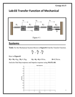
Solution For Task
o Mathematical Equations:- Table#1
For Mass1:-
F = M1 ̈ + k1 x1+ k2 (x1- x2)
= M1 ̈ + k1 x1+ k2x1-k2x2
= ̈ (M1) + x1(k1+ k2)- x2(k2)
For Mass3:-
0 = M3 ̈ +D ̇ + k3 (x3- x2) + k4 x3
= M3 ̈ +D ̇ + k3 x3- k3 x2+ k4 x3
= ̈ (M3) +D ̇ + x3(k3+ k4)- x2(k3)
For Mass2:-
0 = M2 ̈ + k2 (x2- x1) + k3 (x2- x3)
= M2 ̈ + k2 x2- k2 x1+ k3 x2- k3 x3
= ̈ (M2) + x2(k2+ k3)- x1(k2)- x3(k3)
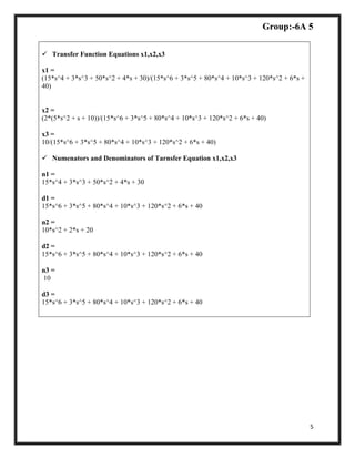
o Transfer Function Equations:- Table#2
For Mass1:-
F = X1(s)[ M1s2
+ k1+ k2]- X2(s)[ k2]
For Mass3:-
0 = -X2(s)[ k3]+ X3(s)[ M3s2
+Ds + k3+ k4]
For Mass2:-
0 = -X1(s)[ k2]+ X2(s)[ M2s2
+ k2+ k3]
- X3(s)[ k3]
Putting values of Mases ,Springs and Damper given in Eq(1), Eq(2), Eq(3).
F = X1(s)[ s2
+ 2]- X2(s)+0 --------------------------Eq(1)
0 = -X1(s)+ X2(s)[1.5s2
+2] - X3(s) --------------------------Eq(2)
0 = 0-X2(s)+ X3(s)[s2
+0.2s+2] --------------------------Eq(3)
o In Matrix Form in MATLAB
[ s^2 + 2, -1, 0]
[ -1, (3*s^2)/2 + 2, -1]
[ 0, -1, s^2 + s/5 + 2]](https://image.slidesharecdn.com/labreport3-171015182314/85/Mathematical-Modelling-of-Electro-Mechanical-System-in-Matlab-2-320.jpg)
![Group:-6A 5
3
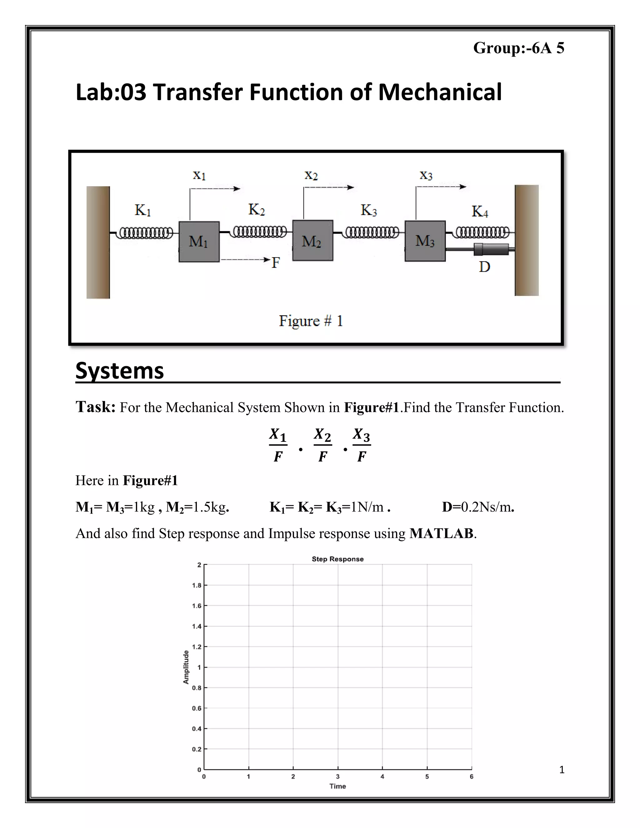
o Code of Task In MATLAB
syms s F X x1 x2 x3 f
X=[x1; x2; x3]
F=[f; 0; 0]
z=[s^2+2 -1 0; -1 1.5*s^2+2 -1; 0 -1 s^2+0.2*s+2]
ZIN=inv(z)
X=ZIN*F
x1=X(1)/f
x2=X(2)/f
x3=X(3)/f
[n1,d1]=numden(x1)
[n2,d2]=numden(x2)
[n3,d3]=numden(x3)
num1=sym2poly(n1);
num2=sym2poly(n2);
num3=sym2poly(n3);
den1=sym2poly(d1);
den2=sym2poly(d2);
den3=sym2poly(d3);
g1=tf(num1,den1);
g2=tf(num2,den2);
g3=tf(num3,den3);
figure
subplot(2,1,1)
step(g1)
title('Step(x1)')
subplot(2,1,2)
impulse(g1)
title('Impulse(x1)')
figure
subplot(2,1,1)
step(g2)
title('Step(x2)')
subplot(2,1,2)
impulse(g2)
title('Impulse(x2)')](https://image.slidesharecdn.com/labreport3-171015182314/85/Mathematical-Modelling-of-Electro-Mechanical-System-in-Matlab-3-320.jpg)
![Group:-6A 5
4
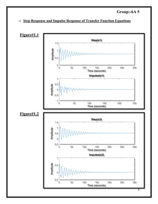
figure
subplot(2,1,1)
step(g3)
title('Step(x3)')
subplot(2,1,2)
impulse(g3)
title('Impulse(x3)')
o Code Result In Command Window
X =
x1
x2
x3
F =
f
0
0
z =
[ s^2 + 2, -1, 0]
[ -1, (3*s^2)/2 + 2, -1]
[ 0, -1, s^2 + s/5 + 2]
ZIN =
[ (15*s^4 + 3*s^3 + 50*s^2 + 4*s + 30)/(15*s^6 + 3*s^5 + 80*s^4 + 10*s^3 + 120*s^2 + 6*s
+ 40), (2*(5*s^2 + s + 10))/(15*s^6 + 3*s^5 + 80*s^4 + 10*s^3 + 120*s^2 + 6*s + 40),
10/(15*s^6 + 3*s^5 + 80*s^4 + 10*s^3 + 120*s^2 + 6*s + 40)]
[ (2*(5*s^2 + s + 10))/(15*s^6 + 3*s^5 + 80*s^4 + 10*s^3 + 120*s^2 + 6*s + 40), (2*(s^2 +
2)*(5*s^2 + s + 10))/(15*s^6 + 3*s^5 + 80*s^4 + 10*s^3 + 120*s^2 + 6*s + 40),
(10*(s^2 + 2))/(15*s^6 + 3*s^5 + 80*s^4 + 10*s^3 + 120*s^2 + 6*s + 40)]
[10/(15*s^6 + 3*s^5 + 80*s^4 + 10*s^3 + 120*s^2 + 6*s + 40), (10*(s^2 +
2))/(15*s^6 + 3*s^5 + 80*s^4 + 10*s^3 + 120*s^2 + 6*s + 40), (5*(3*s^4 + 10*s^2 +
6))/(15*s^6 + 3*s^5 + 80*s^4 + 10*s^3 + 120*s^2 + 6*s + 40)]
X =
(f*(15*s^4 + 3*s^3 + 50*s^2 + 4*s + 30))/(15*s^6 + 3*s^5 + 80*s^4 + 10*s^3 + 120*s^2 +
6*s + 40) (2*f*(5*s^2 + s + 10))/(15*s^6 + 3*s^5 + 80*s^4 + 10*s^3 + 120*s^2 + 6*s + 40)
(10*f)/(15*s^6 + 3*s^5 + 80*s^4 + 10*s^3 + 120*s^2 + 6*s + 40)](https://image.slidesharecdn.com/labreport3-171015182314/85/Mathematical-Modelling-of-Electro-Mechanical-System-in-Matlab-4-320.jpg)
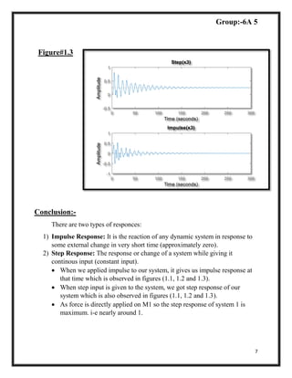

The document outlines the process to find the transfer function of a mechanical system involving three masses and associated forces, springs, and dampers. It includes mathematical equations for each mass and provides MATLAB code for computing the transfer functions along with step and impulse responses. The conclusion highlights the differences between impulse and step responses, showcasing the system's behavior under various inputs.