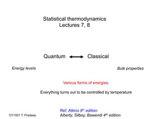
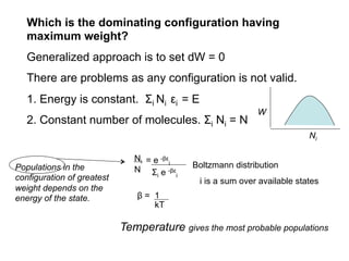
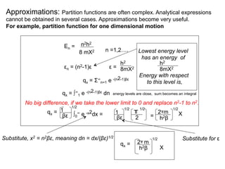
This document discusses statistical thermodynamics and the partition function. It introduces the concept of microscopic configurations and their weights. The Boltzmann distribution relates the probability of a configuration to its weight, which depends on the energy levels and temperature. The partition function allows calculating thermodynamic properties like internal energy, entropy, and heat capacity from knowledge of the energy levels and degeneracies alone. It provides a statistical mechanical approach to thermodynamics.

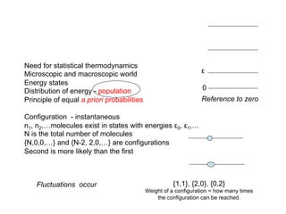
![Energy
0
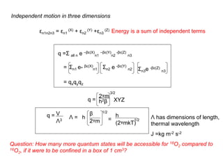
A configuration {3,2,0,0,..} is chosen in 10 different ways - weight of a configuration
How about a general case of N particles ? {n0,n1,…..} configuration of N particles.
A configuration {N-2,2,0,0,…}
First ball of the higher state can be chosen in N ways, because there are N balls
Second ball can be chosen in N-1 ways as there are N-1 balls
But we need to avoid A,B from B,A.
Thus total number of distinguishable configurations is, ½ [N(N-1)]
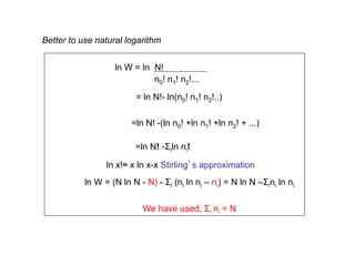
W = N!
W is the weight of the configuration.
How many ways a configuration can be achieved.
n0!n1!n2!....
1 2 3 4 5 6 7 8 9 10
N! ways of selecting balls (first ball N, second (N-1), etc.)
n0! ways of choosing balls in the first level. n1! for the
second, etc.
Distinct ways,
Generalized picture of weight](https://image.slidesharecdn.com/lecture7-8statisticalthermodynamics-introduction-150503014518-conversion-gate01/85/Lecture-7-8-statistical-thermodynamics-introduction-3-320.jpg)
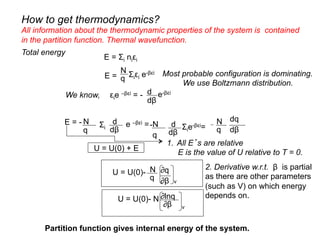
![For a process, change in internal energy, U = U(0) + E
U = U(0) + Σi niεi
How to get entropy?
Internal energy changes occur due to change in populations (Ni + dNi)
or energy states (εi + dεi). Consider a general case:
dU = dU(0) + Σi Ni dεi + Σi εi dNi
For constant volume changes, dU = Σi εi dNi
dU = dqrev = TdS dS = dU/T = k β Σiεi dNi
dS = k Σi(∂lnW/∂ Ni ) dNi + kαΣi dNi
Number of molecules do not change. Second term is zero.
dS = k Σi(∂lnW/∂ Ni ) dNi = k (dlnW)
S = klnW
β εi = (∂lnW/∂Ni ) + α
From the derivation of
Boltzmann distribution
α and β are constants
This can be rewritten (after some manipulations) to
S(T) = [U(T) - U(0)]/T + Nk ln q](https://image.slidesharecdn.com/lecture7-8statisticalthermodynamics-introduction-150503014518-conversion-gate01/85/Lecture-7-8-statistical-thermodynamics-introduction-12-320.jpg)