Download as PDF, PPTX

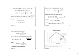
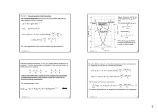

1. The document discusses the quantum states and energy levels of a magnetic model system consisting of N elementary magnets that can point either up or down. 2. There are 2N possible states for the system, and the energy levels are determined by the spin excess, 2m, which is related to the number of up and down spins. The degeneracy of each energy level, g(m), is given by a binomial distribution. 3. For large N, the degeneracy function g(m) takes the form of a sharply peaked Gaussian curve centered around m=0, with a width that decreases with increasing N.


