
Downloaded 19 times
![Statistical Mechanics (P.A. Nagpure) 10
UNIT: II
Distinguishable & Indistinguishable Particles:
In classical mechanics identical particles do not lose their identity despite the similarity of their
physical properties, since individual particles follow sharp trajectories during the course of experiment.
As result classical mechanical particles can be distinguished from one another, hence they are
distinguishable.
As an example consider the molecules of a gas at N.T.P.
Molecular density = 1025
molecules/m3
Therefore volume available for each molecule = 10-25
m3
Molecular radius = 10-10
m
Therefore volume of molecule = 34
3
r =10-30
m3
As the molecule is much smaller than the volume available for it, hence we can identify every molecule
of the gas. Hence they are distinguishable.
In quantum mechanics a particle in motion is represented by a wave packet of finite size and
spread. Hence there is no way of keeping track of individual particles separately, since wave packets of
individual particles considerably overlap to each other. As result quantum mechanical particles cannot be
distinguished from one another, hence they are indistinguishable.
As an example consider the free electrons in metal
Density of free electrons in metal = 1028
m-3
Therefore volume available for each electron = 10-28
m3
For electrons of energy 1eV, the momentum, p = (2mE)1/2
= [2 x 9.1 x 10-31
x 1.6 x 10-19
]1/2
= 0.5 x 10⁻²⁴
kg m/sec
Minimum uncertainty in position of electron,
h
q
p
=
34
9
24
6.63 10
1.3 10
0.5 10
q m
−
−
−
Therefore volume of the wave packet ( )
39 27 34
3.14 1.3 10 10
3
m m− −
Thus, for the free electrons in metal volume available is less than volume of its wave packet. i.e, their
wave packets overlap considerably. Hence free electrons in metal cannot be identified separately. Hence
they are indistinguishable.
Bose-Einstein Statistics:
It is quantum statistics. The particles obeying this statistics are called Bosons. The Bosons are
identical, indistinguishable with spin angular momentum equal to n where, 0,1,2.........n = and there is
no restriction on the number of particles in the quantum state i.e, they do not obey Pauli’s exclusion
principle. The Bosons have symmetric wave function. Examples of Bosons are photons, -particles, -
mesons, etc.
Consider system of particles in equilibrium at absolute temperature T, total energy U, volume V
and total number of particles N.
Let 1 2, ,.... ...i sn n n n be the number of particles in the energy levels 1 2, ,... ...i sE E E E respectively
and 1 2, ,... ...i sg g g g be the number of quantum states associated with the energy levels.
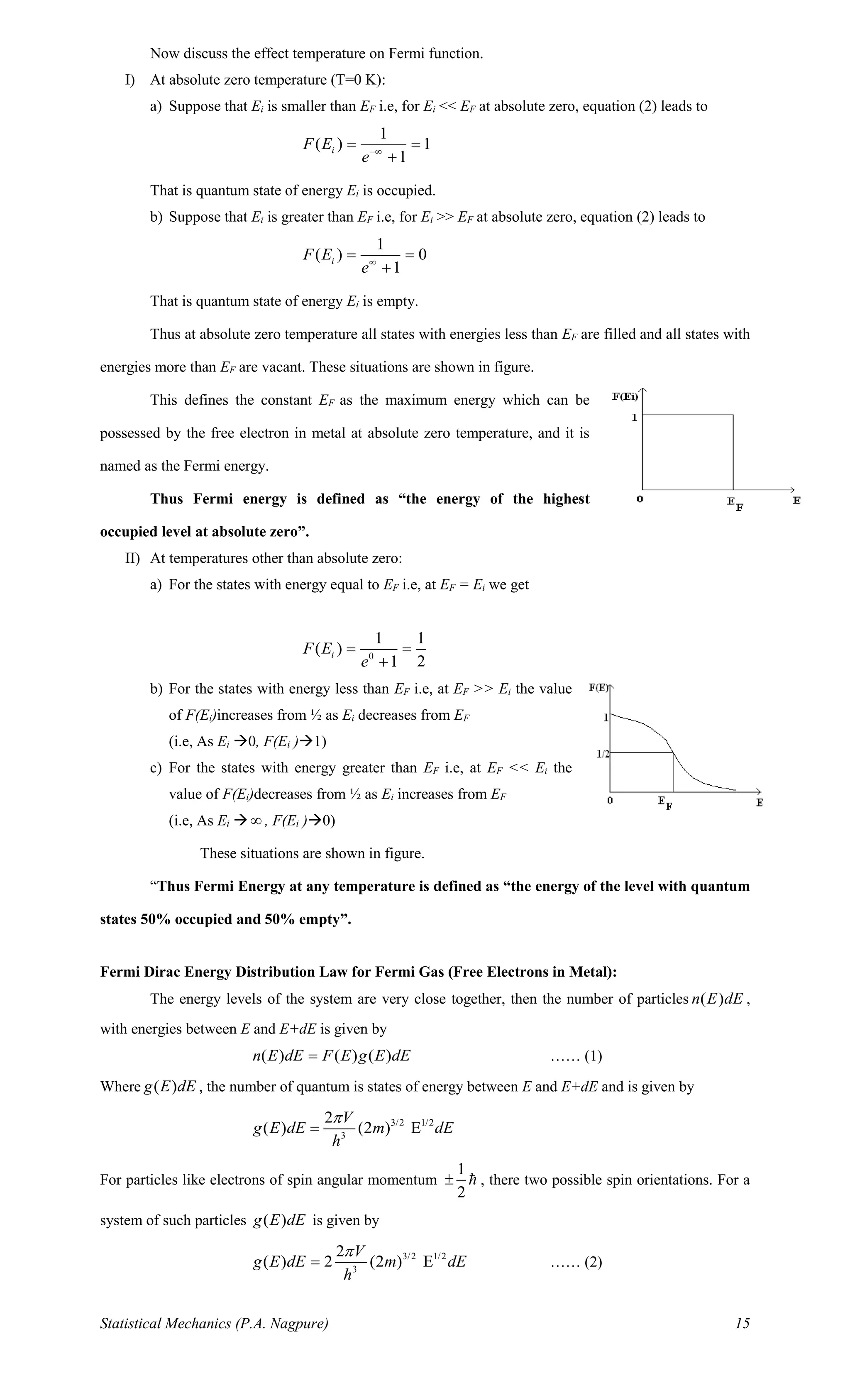
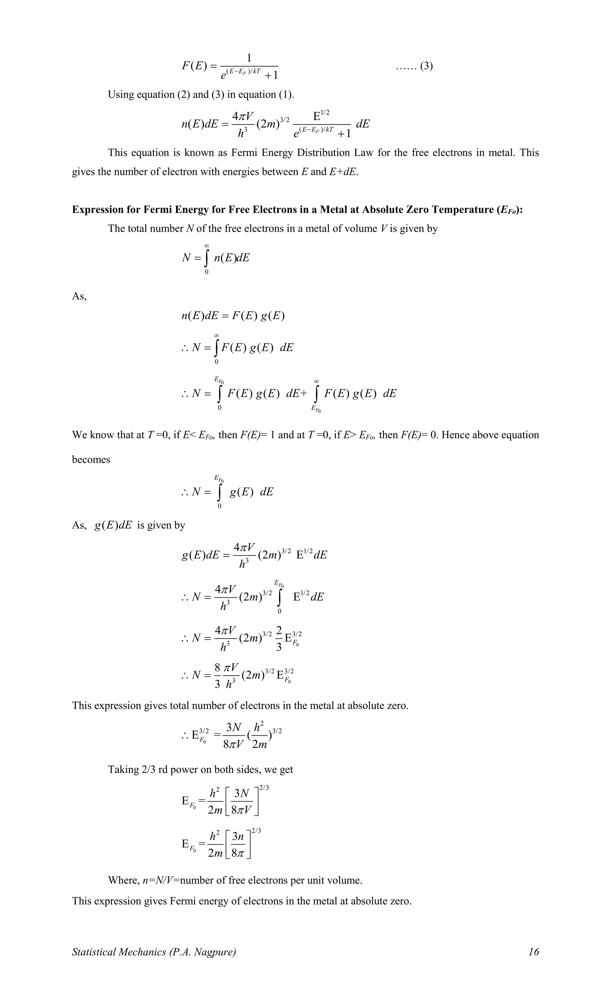
It is evident that,](https://image.slidesharecdn.com/statmech-200412115917/75/Statistical-Mechanics-B-Sc-Sem-VI-10-2048.jpg)
![Statistical Mechanics (P.A. Nagpure) 11
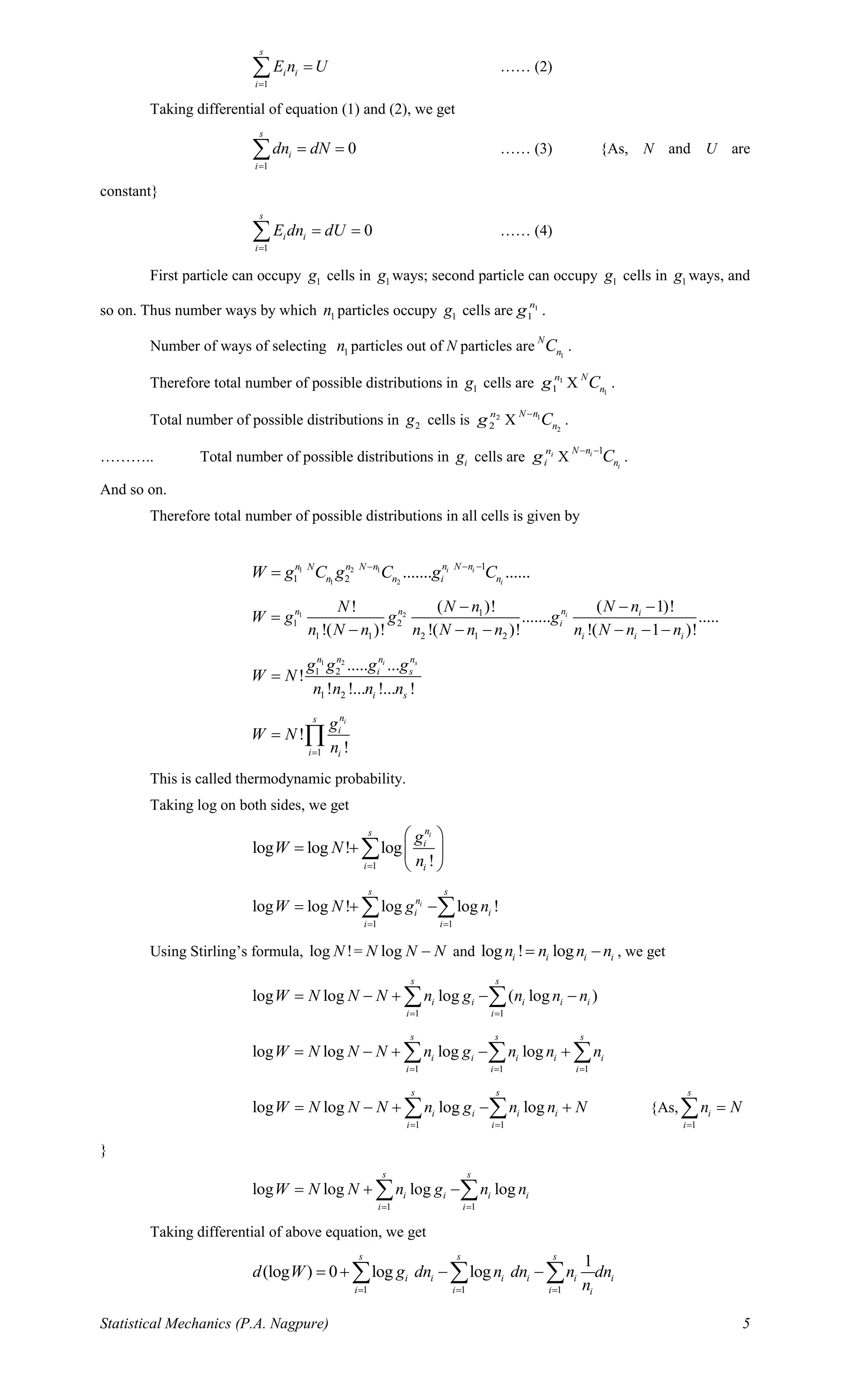
1 2 .... ...i sn n n n N+ + + + + =
1
s
i
i
n N
=
= …… (1)
1 1 2 2 .... ...i i s sE n E n E n E n U+ + + + + =
1
s
i i
i
E n U
=
= …… (2)
Taking differential of equation (1) and (2), we get
1
0
s
i
i
dn dN
=
= = …… (3){As, N and U are constant}
1
0
s
i i
i
E dn dU
=
= = …… (4)
Suppose we have to distribute in indistinguishable particles in ig distinguishable states and there
is no restriction on the number of particles in the quantum state. It is similar to distribute in particles
about ( 1)ig − partitions. The number of possible distributions is
1i i
i
n g
nC+ −
.
Therefore total number of possible distributions of all N particles in all quantum states is given by
1 1 2 2
1 2
1 11 1
....... ........i i S S
i S
n g n gn g n g
n n n nW C C C C+ − + −+ − + −
=
1
1
i i
i
s
n g
n
i
W C+ −
=
=
( )
( )1
1 !
! 1 !
s
i i
i i i
n g
W C
n g=
+ −
=
−
As, 1ig
( )
1
!
! !
s
i i
i i i
n g
W
n g=
+
=
This is called thermodynamic probability.
Taking log on both sides, we get
( )
1
!
log log
! !
s
i i
i i i
n g
W
n g=
+
=
( )
1 1 1
log log ! log ! log !
s s s
i i i i
i i i
W n g n g
= = =
= + − −
Using Stirling’s formula, we get
1 1 1
log [( )log( ) ( )] ( log ) ( log )
s s s
i i i i i i i i i i i i
i i i
W n g n g n g n n n g g g
= = =
= + + − + − − − −
1 1 1 1 1
log ( )log( ) ( ) log ( log )
s s s s s
i i i i i i i i i i i i
i i i i i
W n g n g n g n n n g g g
= = = = =
= + + − + − + − −
Taking differential of above equation, we get](https://image.slidesharecdn.com/statmech-200412115917/75/Statistical-Mechanics-B-Sc-Sem-VI-11-2048.jpg)
This document discusses phase space and the statistical mechanics of classical particles. It can be summarized as: 1. The state of a classical particle is defined by its position and momentum coordinates, which together form a point in the particle's 6D phase space. For a system of N particles, the full 6N-dimensional phase space is called the Γ-space. 2. The minimum volume element in phase space is called the unit cell, with volume h^3 according to Heisenberg's uncertainty principle. 3. The number of quantum states available to particles with energies between E and E+dE is given by the ratio of the volume of phase space to the volume of a unit cell.


