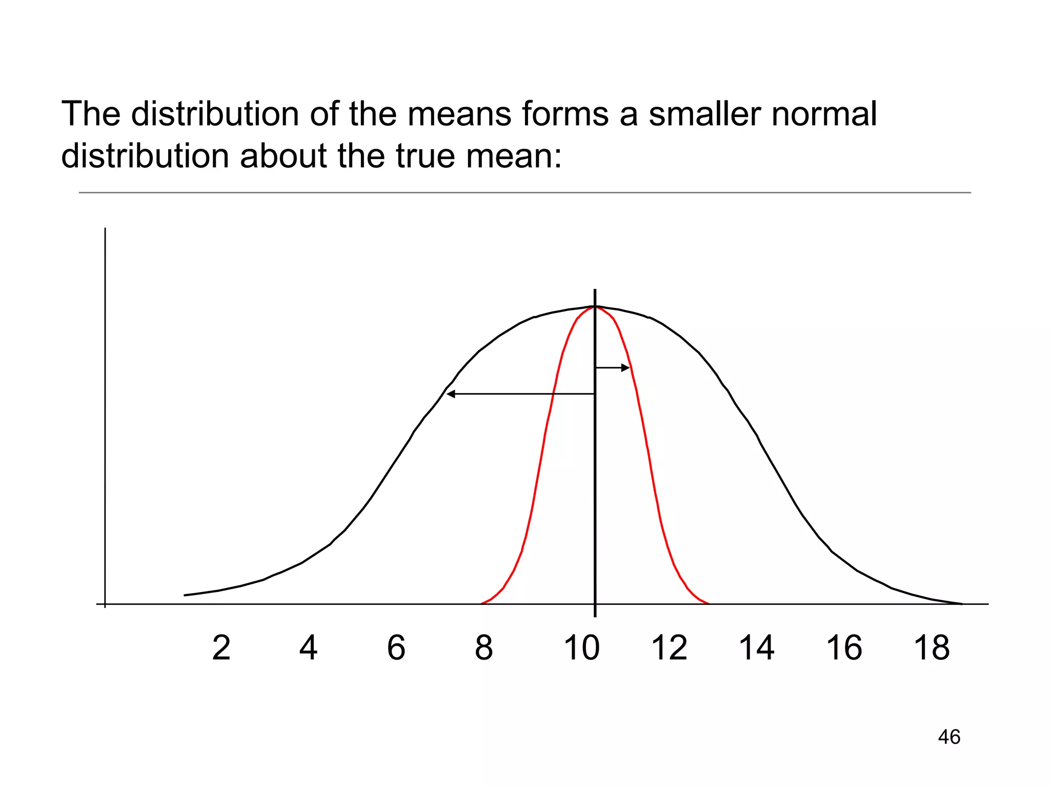
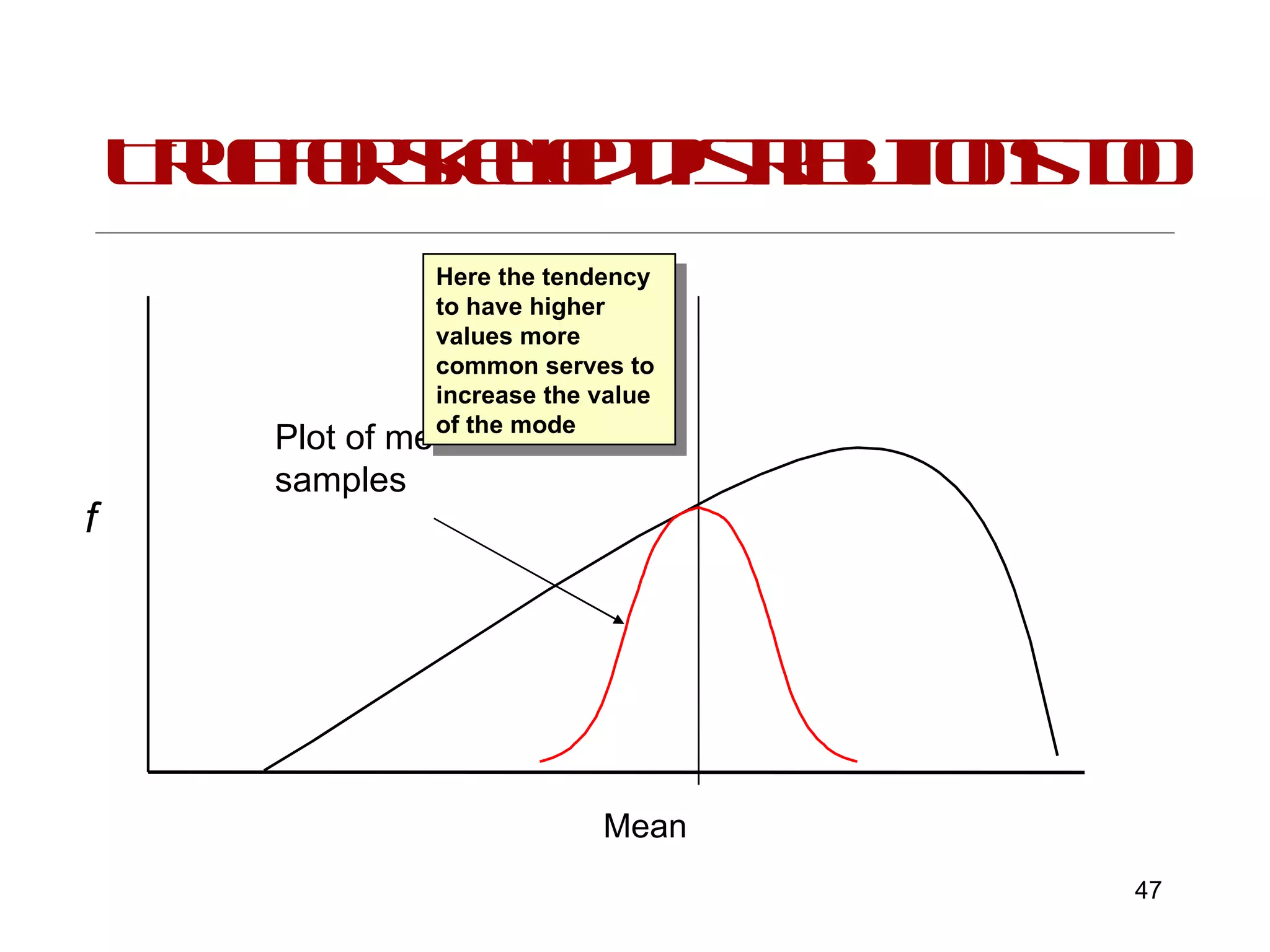
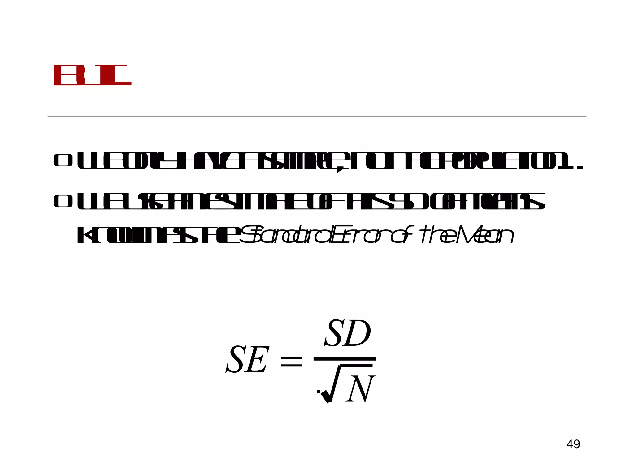
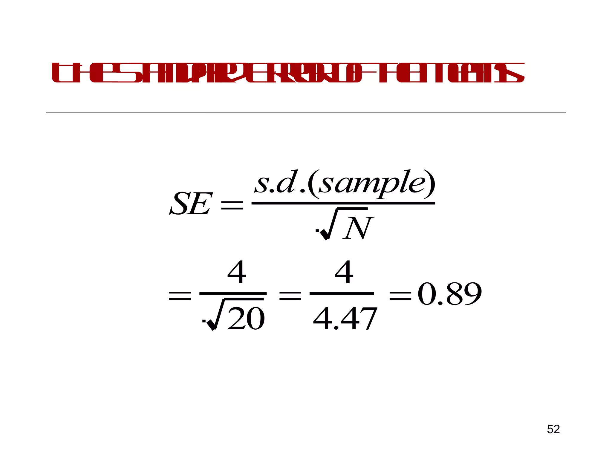
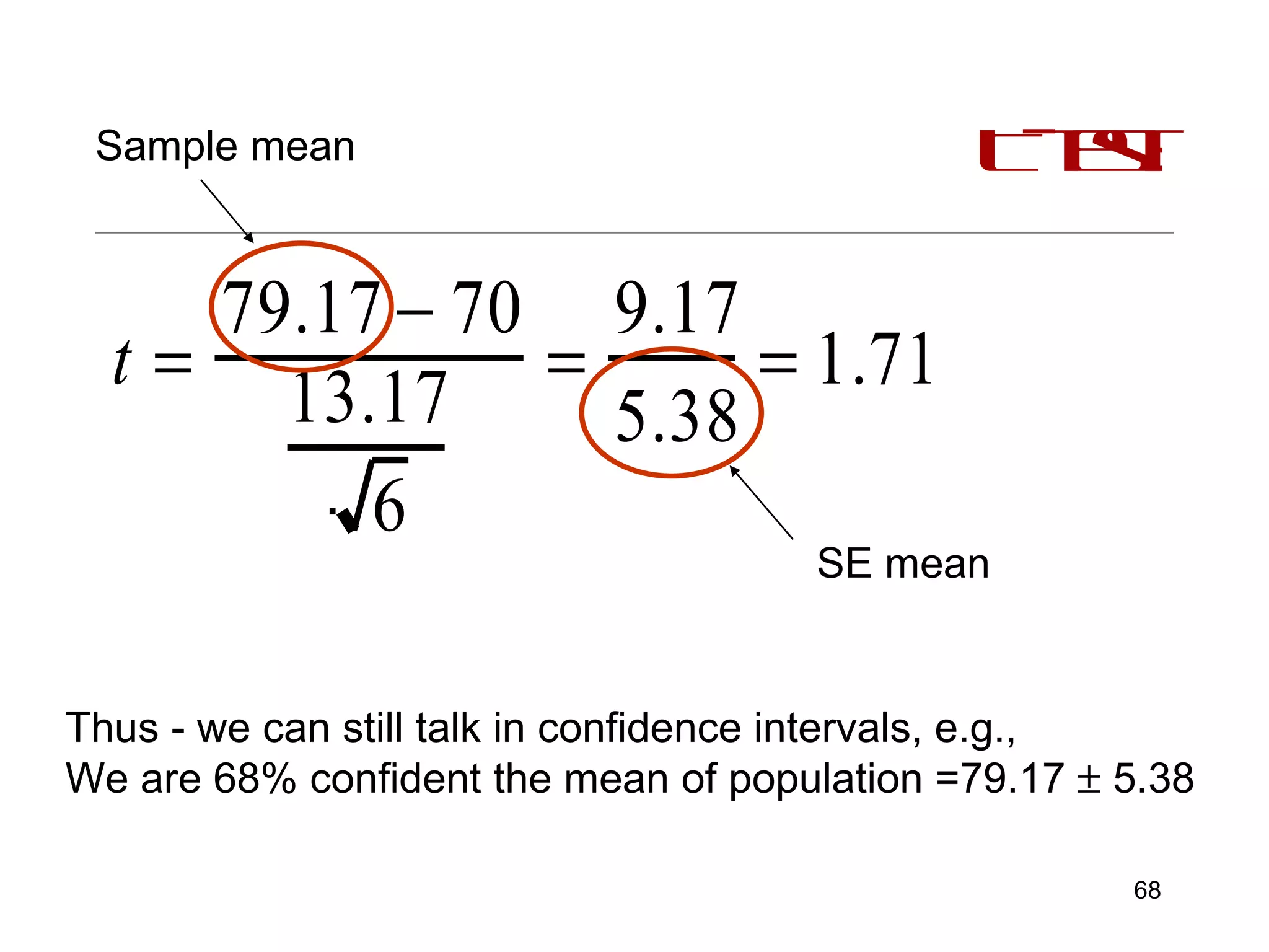
This document provides an introduction to inferential statistics and statistical significance. It discusses key concepts like standard error of the mean, confidence intervals, and comparing means from two samples using a t-test. The document explains how inferential statistics allow researchers to make inferences about populations based on samples and determine if observed differences are likely due to chance or a real effect.

1. Intro to Research in Information Studies Inferential Statistics Standard Error of the Mean Significance Inferential tests you can use

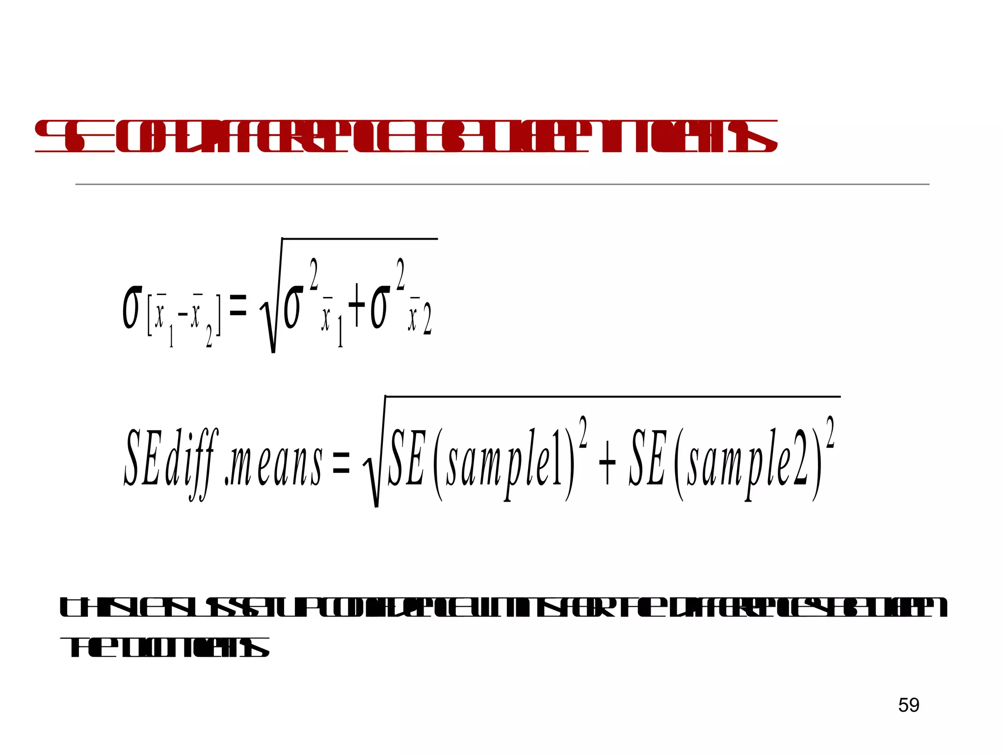
2. Do you speak the language? t = n 1 - X B  2 X B  2 ( ) n 2 - 1 n 1 + ( ) x - ( n 1 -1) + (n 2 -1) X A — X B — X A  2 X A  2 ( ) ( ) ( ) + [ ] 1 n 2

3. Don’t Panic ! t = n 1 - X B  2 X B  2 ( ) n 2 - 1 n 1 + ( ) x - Compare with SD formula ( n 1 -1) + (n 2 -1) Difference between means X A — X B — X A  2 X A  2 ( ) ( ) ( ) + [ ] 1 n 2

4. Basic types of statistical treatment Descriptive statistics which summarize the characteristics of a sample of data Inferential statistics which attempt to say something about a population on the basis of a sample of data - infer to all on the basis of some Statistical tests are inferential

5. Two kinds of descriptive statistic: Measures of central tendency – mean – median – mode Measures of dispersion (variation) – range – inter-quartile range – variance/standard deviation Or where about on the measurement scale most of the data fall Or how spread out they are The different measures have different sensitivity and should be used at the appropriate times…

6. Symbol check Sigma: Means the ‘sum of’ Sigma (1 to n) x of i: means add all values of i from 1 to n in a data set X i = the i th data point

7. Mean Sum of all observations divided by the number of observations In notation: Mean uses every item of data but is sensitive to extreme ‘outliers’ Refer to handout on notation See example on next slide

8. Variance and standard deviation A deviation is a measure of how far from the mean is a score in our data Sample: 6,4,7,5 mean =5.5 Each score can be expressed in terms of distance from 5.5 6,4,7,5, => 0.5, -1.5, 1.5, -0.5 (these are distances from mean) Since these are measures of distance , some are positive (greater than mean) and some are negative (less than the mean) TIP: Sum of these distances ALWAYS = 0 To overcome problems with range etc. we need a better measure of spread

9. Symbol check Called ‘x bar’; refers to the ‘mean’ Called ‘x minus x-bar’; implies subtracting the mean from a data point x. also known as a deviation from the mean

10. Two ways to get SD Sum the sq. deviations from the mean Divide by No. of observations Take the square root of the result Sum the squared raw scores Divide by N Subtract the squared mean Take the square root of the result

11. If we recalculate the variance with the 60 instead of the 5 in the data…

12. If we include a large outlier : Note increase in SD Like the mean, the standard deviation uses every piece of data and is therefore sensitive to extreme values

13. Two sets of data can have the same mean but different standard deviations. The bigger the SD, the more s-p-r-e-a-d out are the data.

14. On the use of N or N-1 When your observations are the complete set of people that could be measured ( parameter ) When you are observing only a sample of potential users ( statistic ), the use of N-1 increases size of sd slightly

15. Summary Mode • Median • Mean • Range • Interquartile Range • Variance / Standard Deviation • Most frequent observation. Use with nominal data ‘ Middle’ of data. Use with ordinal data or when data contain outliers ‘ Average’. Use with interval and ratio data if no outliers Dependent on two extreme values More useful than range. Often used with median Same conditions as mean. With mean, provides excellent summary of data Measures of Central Tendency Measures of Dispersion

16. Deviation units: Z scores Any data point can be expressed in terms of its Distance from the mean in SD units: A positive z score implies a value above the mean A negative z score implies a value below the mean Andrew Dillon: Move this to later in the course, after distributions?

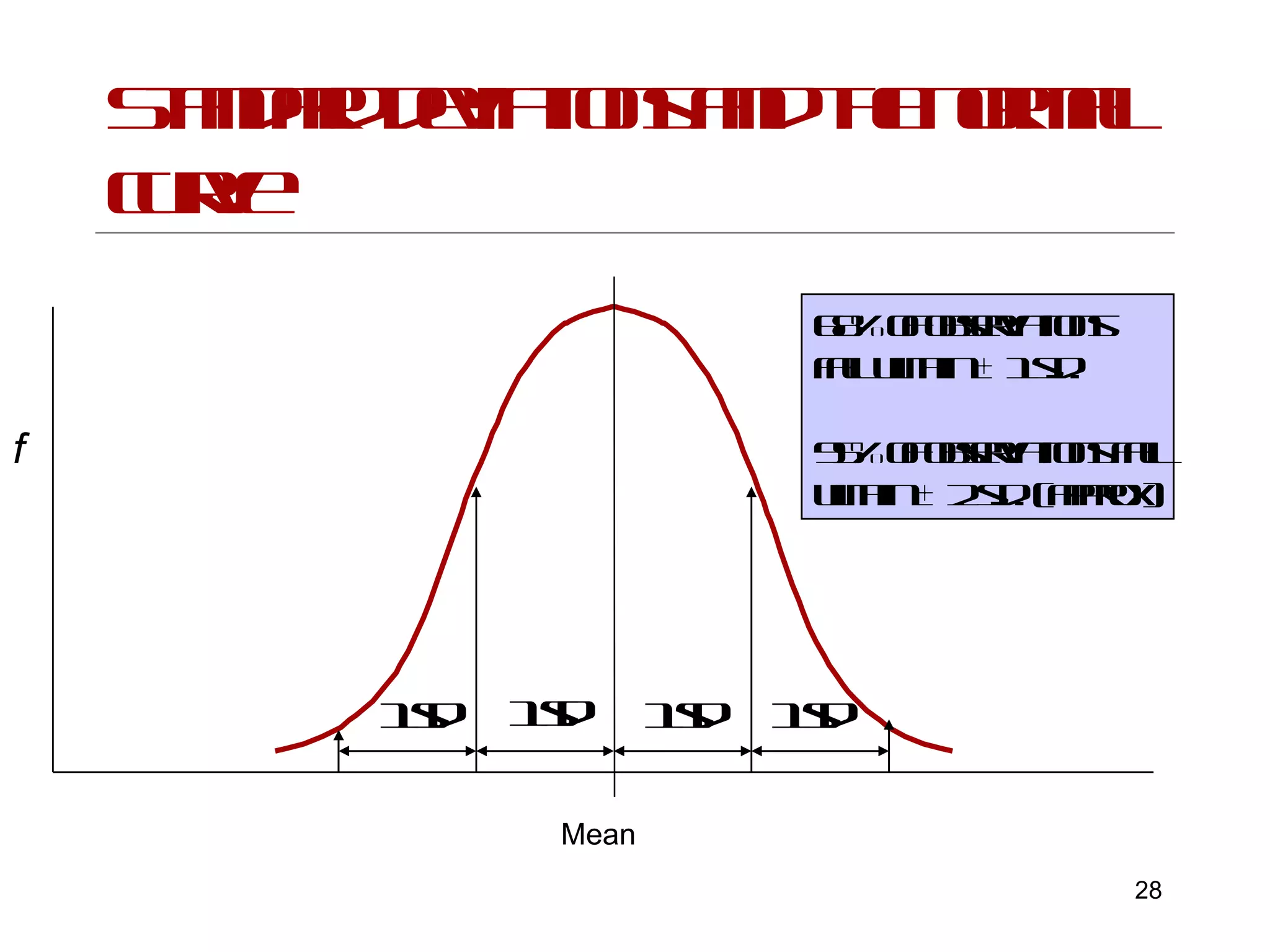
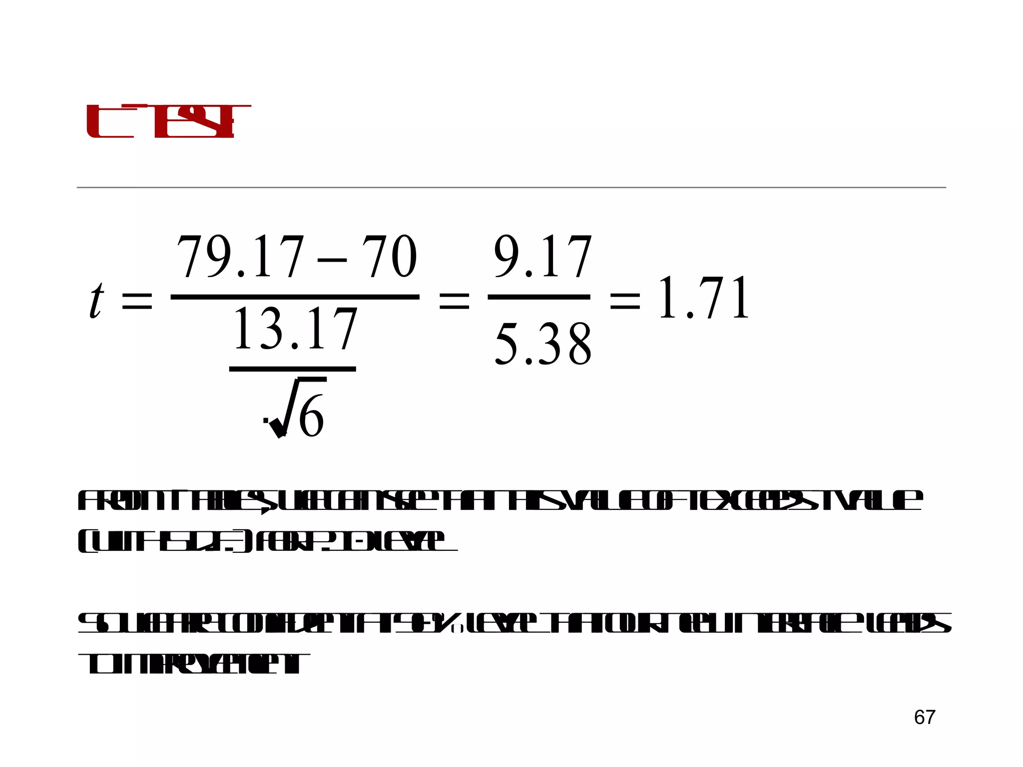
17. Interpreting Z scores Mean = 70,SD = 6 Then a score of 82 is 2 sd [ (82-70)/6] above the mean, or 82 = Z score of 2 Similarly, a score of 64 = a Z score of -1 By using Z scores, we can standardize a set of scores to a scale that is more intuitive Many IQ tests and aptitude tests do this, setting a mean of 100 and an SD of 10 etc.

18. Comparing data with Z scores You score 49 in class A but 58 in class B How can you compare your performance in both? Class A: Class B: Mean =45 Mean =55 SD=4 SD = 6 49 is a Z=1.0 58 is a Z=0.5

19. With normal distributions Mean, SD and Z tables In combination provide powerful means of estimating what your data indicates

20. Graphing data - the histogram Number Of errors The categories of data we are studying, e.g., task or interface, or user group etc. The frequency of occurrence for measure of interest, e.g., errors, time, scores on a test etc. 1 2 3 4 5 6 7 8 9 10 Graph gives instant summary of data - check spread, similarity, outliers, etc.

21. Very large data sets tend to have distinct shape:

22. Normal distribution Bell shaped, symmetrical, measures of central tendency converge mean, median, mode are equal in normal distribution Mean lies at the peak of the curve Many events in nature follow this curve IQ test scores, height, tosses of a fair coin, user performance in tests,

23. The Normal Curve NB: position of measures of central tendency Mean Median Mode 50% of scores fall below mean f

24. Positively skewed distribution Note how the various measures of central tendency separate now - note the direction of the change…mode moves left of other two, mean stays highest, indicating frequency of scores less than the mean Mode Median Mean f

25. Negatively skewed distribution Here the tendency to have higher values more common serves to increase the value of the mode Mean Median Mode f

26. Other distributions Bimodal Data shows 2 peaks separated by trough Multimodal More than 2 peaks The shape of the underlying distribution determines your choice of inferential test

27. Bimodal f Mean Median Mode Mode Will occur in situations where there might be distinct groups being tested e.g., novices and experts Note how each mode is itself part of a normal distribution (more later)

28. Standard deviations and the normal curve Mean 1 sd f 1 sd 68% of observations fall within ± 1 s.d. 95% of observations fall within ± 2 s.d. (approx) 1 sd 1 sd

29. Z scores and tables Knowing a Z score allows you to determine where under the normal distribution it occurs Z score between: 0 and 1 = 34% of observations 1 and -1 = 68% of observations etc. Or 16% of scores are >1 Z score above mean Check out Z tables in any basic stats book

30. Remember: A Z score reflects position in a normal distribution The Normal Distribution has been plotted out such that we know what proportion of the distribution occurs above or below any point

31. Importance of distribution Given the mean, the standard deviation, and some reasonable expectation of normal distribution, we can establish the confidence level of our findings With a distribution, we can go beyond descriptive statistics to inferential statistics (tests of significance)

32. So - for your research: Always summarize the data by graphing it - look for general pattern of distribution Then, determine the mean, median, mode and standard deviation From these we know a LOT about what we have observed

33. Inference is built on Probability Inferential statistics rely on the laws of probability to determine the ‘significance’ of the data we observe. Statistical significance is NOT the same as practical significance In statistics, we generally consider ‘significant’ those differences that occur less than 1:20 by chance alone

34. Calculating probability Probability refers to the likelihood of any given event occurring out of all possible events e.g.: Tossing a coin - outcome is either head or tail Therefore probability of head is 1/2 Probability of two heads on two tosses is 1/4 since the other possible outcomes are two tails, and two possible sequences of head and tail. The probability of any event is expressed as a value between 0 (no chance) and 1 (certain) At this point I ask people to take out a coin and toss it 10 times, noting the exact sequence of outcomes e.g., h,h,t,h,t,t,h,t,t,h. Then I have people compare outcomes….

35. Sampling distribution for 3 coin tosses

36. Probability and normal curves Q? When is the probability of getting 10 heads in 10 coin tosses the same as getting 6 heads and 4 tails? HHHHHHHHHH HHTHTHHTHT Answer: when you specify the precise order of the 6 H/4T sequence: (1/2) 10 =1/1024 (specific order) But to get 6 heads, in any order it is: 210/1024 (or about 1:5)

37. What use is probability to us? It tells us how likely is any event to occur by chance This enables us to determine if the behavior of our users in a test is just chance or is being affected by our interfaces

38. Determining probability Your statistical test result is plotted against the distribution of all scores on such a test. It can be looked up in stats tables or is calculated for you in EXCEL or SPSS etc This tells you its probability of occurrence The distributions have been determined by statisticians. Introduce simple stats tables here :

39. What is a significance level? In research, we estimate the probability level of finding what we found by chance alone. Convention dictates that this level is 1:20 or a probability of .05, usually expressed as : p<.05. However, this level is negotiable But the higher it is (e.g., p<.30 etc) the more likely you are to claim a difference that is really just occurring by chance (known as a Type 1 error)

40. What levels might we chose? In research there are two types of errors we can make when considering probability: Claiming a significant difference when there is none (type 1 error) Failing to claim a difference where there is one (type 2 error) The p<.05 convention is the ‘balanced’ case but tends to minimize type 1 errors

41. Using other levels Type 1 and 2 errors are interwoven, if we lessen the probability of one occurring, we increase the chance of the other. If we think that we really want to find any differences that exist, we might accept a probability level of .10 or higher

42. Thinking about p levels The p<.x level means we believe our results could occur by chance alone (not because of our manipulation) at least x/100 times P<.10 => our results should occur by chance 1 in 10 times P<.20=> our results should occur by chance 2 in 10 times Depending on your context, you can take your chances :) In research, the consensus is 1:20 is high enough…..

43. Putting probability to work Understanding the probability of gaining the data you have can guide your decisions Determine how precise you need to be IN ADVANCE, not after you see the result It is like making a bet….you cannot play the odds after the event!

44. Sampling error and the mean Usually, our data forms only a small part of all the possible data we could collect All possible users do not participate in a usability test Every possible respondent did not answer our questions The mean we observe therefore is unlikely to be the exact mean for the whole population The scores of our users in a test are not going to be an exact index of how all users would perform I find that this is the hardest part of stats for novices to grasp, since it is the bridge between descriptive and inferential stats…..needs to be explained slowly!!

45. How can we relate our sample to everyone else? Central limit theorem If we repeatedly sample and calculate means from a population, our list of means will itself be normally distributed Holds true even for samples taken from a skewed population distribution This implies that our observed mean follows the same rules as all data under the normal curve

46. 2 4 6 8 10 12 14 16 18 The distribution of the means forms a smaller normal distribution about the true mean:

47. True for skewed distributions too Mean f Plot of means from samples Here the tendency to have higher values more common serves to increase the value of the mode

48. How means behave.. A mean of any sample belongs to a normal distribution of possible means of samples Any normal distribution behaves lawfully If we calculate the SD of all these means, we can determine what proportion (%) of means fall within specific distances of the ‘true’ or population mean

49. But... We only have a sample, not the population… We use an estimate of this SD of means known as the Standard Error of the Mean

50. Implications Given a sample of data, we can estimate how confident we are in it being a true reflection of the ‘world’ or… If we test 10 users on an interface or service, we can estimate how much variability about our mean score we will find within the intended full population of users

51. Example We test 20 users on a new interface: Mean error score: 10, sd: 4 What can we infer about the broader user population? According to the central limit theorem, our observed mean (10 errors) is itself 95% likely to be within 2 s.d. of the ‘true’ (but unknown to us) mean of the population

52. The Standard Error of the Means

53. If standard error of mean = 0.89 Then observed (sample) mean is within a normal distribution about the ‘true’ or population mean: So we can be 68% confident that the true mean=10  0.89 95% confident our population mean = 10  1.78 99% confident it is within 10  2.67 This offers a strong method of interpreting of our data

54. Issues to note If s.d. is large and/or sample size is small, the estimated deviation of the population means will appear large. e.g., in last example, if n=9, SE mean=1.33 So confidence interval becomes 10  2.66 (i.e., we are now 95% confident that the true mean is somewhere between 7.34 and 12.66. Hence confidence improves as sample increases and variability lessens Or in other words: the more users you study, the more sure you can be….!

55. Exercise: If the mean = 10 and the s.d.=4, what is the 68% confidence interval when we have: 16 users? 9 users? If the s.d. = 12, and mean is still 10, what is the 95% confidence interval for those N? Answers: 9-11 8.66-11.33 4-16 2-18

56. Exercise answers: If the mean = 10 and the s.d.=4, what is the 68% confidence interval when we have: 16 users?= 9-11 (hint: sd/  n = 4/4=1) 9 users? = 8.66-11.33 If the s.d. = 12, and mean is still 10, what is the 95% confidence interval for those N? 16 users: 4-16 (hint: 95% CI implies 2 SE either side of mean) 9 users: 2-18

57. Recap Summarizing data effectively informs us of central tendencies We can estimate how our data deviates from the population we are trying to estimate We can establish confidence intervals to enable us to make reliable ‘bets’ on the effects of our designs on users

58. Comparing 2 means The differences between means of samples drawn from the same population are also normally distributed Thus, if we compare means from two samples, we can estimate if they belong to the same parent population This is the beginning of significance testing

59. SE of difference between means This lets us set up confidence limits for the differences between the two means

60. Regardless of population mean: The difference between 2 true measures of the mean of a population is 0 The differences between pairs of sample means from this population is normally distributed about 0

61. Consider two interfaces: We capture 10 users’ times per task on each. The results are: Interface A = mean 8, sd =3 Interface B = mean 10, sd=3.5 Q? - is Interface A really different? How do we tackle this question?

62. Calculate the SE difference between the means SE a = 3/  10 = 0.95 SE b = 3.5/  10=1.11 SE a-b =  (0.95 2 +1.11 2 ) =  (0.90+1.23)=1.46 Observed Difference between means= 2.0 95% Confidence interval of difference between means is 2 x(1.46) or 2.92 (i.e. we expect to find difference between 0-2.92 by chance alone). suggests there is no significant difference at the p<.05 level.

63. But what else? We can calculate the exact probability of finding this difference by chance: Divide observed difference between the means by the SE( diff between means ): 2.0/1.46 = 1.37 Gives us the number of standard deviation units between two means (Z scores) Check Z table: 82% of observations are within 1.37 sd, 18% are greater; thus the precise sig level of our findings is p<.18. Thus - Interface A is different, with rough odds of 5:1

64. Hold it! Didn’t we first conclude there was no significant difference? Yes, no significant difference at p<.05 But the probability of getting the differences we observed by chance was approximately 0.18 Not good enough for science (must avoid type 1 error), but very useful for making a judgment on design But you MUST specify levels you will accept BEFORE not after…. Note - for small samples (n<20) t- distribution is better than z distribution, when looking up probability

65. Why t? Similar to the normal distribution t distribution is flatter than Z for small degrees of freedom (n-1), but virtually identical to Z when N>30 Exact shape of t-distribution depends on sample size

66. Simple t-test: You want all users of a new interface to score at least 70% on an effectiveness test. You test 6 users on a new interface and gain the following scores: 62 92 75 68 83 95 Mean = 79.17 Sd=13.17

67. T-test: From t-tables, we can see that this value of t exceeds t value (with 5 d.f.) for p.10 level So we are confident at 90% level that our new interface leads to improvement

68. T-test: SE mean Sample mean Thus - we can still talk in confidence intervals, e.g., We are 68% confident the mean of population =79.17  5.38

69. Predicting the direction of the difference Since you stated that you wanted to see if new Interface was BETTER (>70), not just DIFFERENT (< or > 70%), this is asking for a one-sided test…. For a two-sided test, I just want to see if there is ANY difference (better or worse) between A and B.

70. One tail (directional) test Tester narrows the odds by half by testing for a specific difference One sided predictions specify which part of the normal curve the difference observed must reside in (left or right) Testing for ANY difference is known as ‘two-tail’ testing, Testing for a directional difference (A>B) is known as ‘one-tail’ testing

71. So to recap If you are interested only in certain differences, you are being ‘directional’ or ‘one-sided’ Under the normal curve, random or chance differences occur equally on both sides You MUST state directional expectations (hypothesis) in advance

72. Why would you predict the direction? Theoretical grounds Experience or previous findings suggested the difference Practical grounds You redesigned the interface to make it better, so you EXPECT users will perform better….