Les5e ppt 06

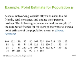
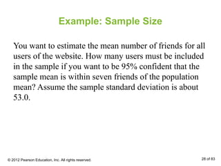
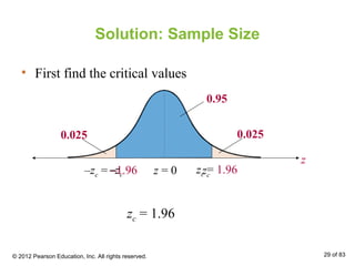
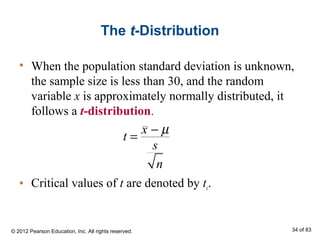
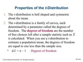
Chapter
Confidence Intervals
1 of 83
6
© 2012 Pearson Education, Inc.
All rights reserved.

Chapter Outline
• 6.1 Confidence Intervals for the Mean (Large
Samples)
• 6.2 Confidence Intervals for the Mean (Small
Samples)
• 6.3 Confidence Intervals for Population Proportions
• 6.4 Confidence Intervals for Variance and Standard
Deviation
© 2012 Pearson Education, Inc. All rights reserved. 2 of 83

Section 6.1
Confidence Intervals for the Mean
(Large Samples)

Section 6.1 Objectives
• Find a point estimate and a margin of error
• Construct and interpret confidence intervals for the
population mean
• Determine the minimum sample size required when
estimating μ

Point Estimate for Population μ
Point Estimate
• A single value estimate for a population parameter
• Most unbiased point estimate of the population mean
μ is the sample mean x
Estimate Population
Parameter…
with Sample
Statistic
Mean: μ x

Example: Point Estimate for Population μ
A social networking website allows its users to add
friends, send messages, and update their personal
profiles. The following represents a random sample of
the number of friends for 40 users of the website. Find a
point estimate of the population mean, µ. (Source:
Facebook)
140 105 130 97 80 165 232 110 214 201 122
98 65 88 154 133 121 82 130 211 153 114
58 77 51 247 236 109 126 132 125 149 122
74 59 218 192 90 117 105

Solution: Point Estimate for Population μ
The sample mean of the data is
5232
130.8
40
x
x
n
Σ
= = =
Your point estimate for the mean number of friends for
all users of the website is 130.8 friends.

115 120 125 130 135 140 150145
Point estimate
115 120 125 130 135 140 150145
Point estimate
130.8x =
How confident do we want to be that the interval estimate
contains the population mean μ?
Interval Estimate
Interval estimate
• An interval, or range of values, used to estimate a
population parameter.
( )
Interval estimate
Right endpoint
146.5
Left endpoint
115.1

Level of Confidence
Level of confidence c
• The probability that the interval estimate contains the
population parameter.
z
z = 0–zc zc
Critical values
½(1 – c) ½(1 – c)
c is the area under the
standard normal curve
between the critical values.
The remaining area in the tails is 1 – c .
c
Use the Standard
Normal Table to find the
corresponding z-scores.

−zc
Level of Confidence
• If the level of confidence is 90%, this means that we
are 90% confident that the interval contains the
population mean μ.
z
z = 0 zc
The corresponding z-scores are ±1.645.
c = 0.90
½(1 – c) = 0.05½(1 – c) = 0.05
–zc = –1.645 zc = 1.645

Sampling Error
Sampling error
• The difference between the point estimate and the
actual population parameter value.
• For μ:
 the sampling error is the difference – μ
 μ is generally unknown
 varies from sample to sample
x
x

Margin of Error
Margin of error
• The greatest possible distance between the point
estimate and the value of the parameter it is
estimating for a given level of confidence, c.
• Denoted by E.
• Sometimes called the maximum error of estimate or
error tolerance.
c x cE z z
n
= =
σσ When n ≥ 30, the sample
standard deviation, s, can
be used for σ.

Example: Finding the Margin of Error
Use the social networking website data and a 95%
confidence level to find the margin of error for the
mean number of friends for all users of the website.
Assume the sample standard deviation is about 53.0.

−zc
Solution: Finding the Margin of Error
• First find the critical values
z
zcz = 0
0.95
0.0250.025
–zc = –1.96
95% of the area under the standard normal curve falls
within 1.96 standard deviations of the mean. (You
can approximate the distribution of the sample means
with a normal curve by the Central Limit Theorem,
because n = 40 ≥ 30.)
zc = 1.96

Solution: Finding the Margin of Error
53.0
1.96
40
16.4
c c
s
E z z
n n
σ
≈
=
×
≈
≈
You don’t know σ, but
since n ≥ 30, you can
use s in place of σ.
You are 95% confident that the margin of error for the
population mean is about 16.4 friends.

Confidence Intervals for the Population
Mean
A c-confidence interval for the population mean μ
•
• The probability that the confidence interval contains
μ is c.
where cx E x E E z
n
σ
µ− < < + =

Constructing Confidence Intervals for μ
Finding a Confidence Interval for a Population Mean
(n ≥ 30 or σ known with a normally distributed population)
In Words In Symbols
1. Find the sample statistics n and
.
2. Specify σ, if known.
Otherwise, if n ≥ 30, find the
sample standard deviation s and
use it as an estimate for σ.
x
x
n
Σ
=
2
( )
1
x x
s
n
Σ −
=
−
x

Constructing Confidence Intervals for μ
3. Find the critical value zc that
corresponds to the given
level of confidence.
4. Find the margin of error E.
5. Find the left and right
endpoints and form the
confidence interval.
Use the Standard
Normal Table or
technology.
Left endpoint:
Right endpoint:
Interval:
cE z
n
σ
=
x E−
x E+
x E x Eµ− < < +
In Words In Symbols

Example: Constructing a Confidence
Interval
Construct a 95% confidence interval for the mean
number of friends for all users of the website.
Solution: Recall and E ≈ 16.4130.8x =
130.8 16.4
114.4
x E−
≈ −
=
130.8 16.4
147.2
x E+
≈ +
=
114.4 < μ < 147.2
Left Endpoint: Right Endpoint:

Solution: Constructing a Confidence
Interval
114.4 < μ < 147.2
•
With 95% confidence, you can say that the
population mean number of friends is between 114.4
and 147.2.

Interval σ Known
A college admissions director wishes to estimate the
mean age of all students currently enrolled. In a random
sample of 20 students, the mean age is found to be 22.9
years. From past studies, the standard deviation is
known to be 1.5 years, and the population is normally
distributed. Construct a 90% confidence interval of the
population mean age.

−zc
Interval σ Known
z
z = 0 zc
c = 0.90
½(1 – c) = 0.05½(1 – c) = 0.05
–zc = –1.645 zc = 1.645
zc = 1.645

• Margin of error:
• Confidence interval:
Interval σ Known
1.5
1.645 0.6
20
cE z
n
σ
= ≈= ×
22.9 0.6
22.3
x E−
≈ −
=
22.9 0.6
23.5
x E+
≈ +
=
22.3 < μ < 23.5

Interval σ Known
22.3 < μ < 23.5
( )•
22.922.3 23.5
With 90% confidence, you can say that the mean age
of all the students is between 22.3 and 23.5 years.
Point estimate
xx E− x E+

Interpreting the Results
• μ is a fixed number. It is either in the confidence
interval or not.
• Incorrect: “There is a 90% probability that the actual
mean is in the interval (22.3, 23.5).”
• Correct: “If a large number of samples is collected
and a confidence interval is created for each sample,
approximately 90% of these intervals will contain μ.

Interpreting the Results
The horizontal segments
represent 90% confidence
intervals for different
samples of the same size.
In the long run, 9 of every
10 such intervals will
contain μ. μ

Sample Size
• Given a c-confidence level and a margin of error E,
the minimum sample size n needed to estimate the
population mean µ is
• If σ is unknown, you can estimate it using s, provided
you have a preliminary sample with at least 30
members.
2
cz
n
E
σ 
=  ÷
 

Example: Sample Size
You want to estimate the mean number of friends for all
users of the website. How many users must be included
in the sample if you want to be 95% confident that the
sample mean is within seven friends of the population
mean? Assume the sample standard deviation is about
53.0.

−zc
Solution: Sample Size
zc = 1.96
z
z = 0 zc
0.95
0.0250.025
–zc = –1.96 zc = 1.96

zc = 1.96 σ ≈ s ≈ 53.0 E = 7
2 2
1.96 53.0
220.23
7
cz
n
E
σ × 
≈ ≈
 
=  ÷



÷
 
When necessary, round up to obtain a whole number.
You should include at least 221 users in your sample.

Section 6.1 Summary
• Found a point estimate and a margin of error
• Constructed and interpreted confidence intervals for
the population mean
• Determined the minimum sample size required when
estimating μ

Section 6.2
Confidence Intervals for the Mean
(Small Samples)

• Interpret the t-distribution and use a t-distribution
table
• Construct confidence intervals when n < 30, the
population is normally distributed, and σ is unknown

The t-Distribution
• When the population standard deviation is unknown,
the sample size is less than 30, and the random
variable x is approximately normally distributed, it
follows a t-distribution.
• Critical values of t are denoted by tc.
t =
x − µ
s
n

Properties of the t-Distribution
1. The t-distribution is bell shaped and symmetric
about the mean.
2. The t-distribution is a family of curves, each
determined by a parameter called the degrees of
freedom. The degrees of freedom are the number
of free choices left after a sample statistic such as
is calculated. When you use a t-distribution to
estimate a population mean, the degrees of freedom
are equal to one less than the sample size.
 d.f. = n – 1 Degrees of freedom
x

Properties of the t-Distribution
3. The total area under a t-curve is 1 or 100%.
4. The mean, median, and mode of the t-distribution are
equal to zero.
5. As the degrees of freedom increase, the t-distribution
approaches the normal distribution. After 30 d.f., the t-
distribution is very close to the standard normal z-
distribution.
t
0
Standard normal curve
The tails in the t-
distribution are “thicker”
than those in the standard
normal distribution.d.f. = 5
d.f. = 2

Example: Critical Values of t
Find the critical value tc for a 95% confidence level
when the sample size is 15.
Table 5: t-Distribution
tc = 2.145
Solution: d.f. = n – 1 = 15 – 1 = 14

Solution: Critical Values of t
95% of the area under the t-distribution curve with 14
degrees of freedom lies between t = ±2.145.
t
–tc = –2.145 tc = 2.145
c = 0.95

Confidence Intervals for the Population
Mean
A c-confidence interval for the population mean μ
•
• The probability that the confidence interval contains
μ is c.
where c
s
x E x E E t
n
µ− < < + =

Confidence Intervals and t-Distributions
1. Identify the sample
statistics n, , and s.
2. Identify the degrees of
freedom, the level of
confidence c, and the
critical value tc.
x
x
n
Σ
=
2
( )
1
x x
s
n
∑ −
=
−
cE t
n
=
s
d.f. = n – 1
x
In Words In Symbols

Confidence Intervals and t-Distributions
Left endpoint:
Right endpoint:
Interval:
x E−
x E+
x E x Eµ− < < +
In Words In Symbols

Interval
You randomly select 16 coffee shops and measure the
temperature of the coffee sold at each. The sample mean
temperature is 162.0ºF with a sample standard deviation
of 10.0ºF. Find the 95% confidence interval for the
population mean temperature. Assume the temperatures
are approximately normally distributed.
Solution:
Use the t-distribution (n < 30, σ is unknown,
temperatures are approximately normally distributed).

Interval
• n =16, x = 162.0 s = 10.0 c = 0.95
• df = n – 1 = 16 – 1 = 15
• Critical Value Table 5: t-Distribution
tc = 2.131

Interval
10
2.131 5.3
16
cE t
n
= = × ≈
s
162 5.3
156.7
x E−
≈ −
=
162 5.3
167.3
x E+
≈ +
=
156.7 < μ < 167.3

Interval
• 156.7 < μ < 167.3
( )•
162.0156.7 167.3
population mean temperature of coffee sold is
between 156.7ºF and 167.3ºF.
Point estimate
xx E− x E+

No
Normal or t-Distribution?
Is n ≥ 30?
Is the population normally,
or approximately
normally, distributed? Cannot use the normal
distribution or the t-distribution.
Yes
Is σ known?
No
Use the normal distribution with
If σ is unknown, use s instead.
cE z
n
=
σ
Yes
No
Use the normal distribution with
.cE z
n
=
σ
Yes
Use the t-distribution with
and n – 1 degrees of freedom.
cE t
n
=
s

Example: Normal or t-Distribution?
You randomly select 25 newly constructed houses. The
sample mean construction cost is $181,000 and the
population standard deviation is $28,000. Assuming
construction costs are normally distributed, should you
use the normal distribution, the t-distribution, or neither
to construct a 95% confidence interval for the
population mean construction cost?
Solution:
Use the normal distribution (the population is
normally distributed and the population standard
deviation is known)

Section 6.2 Summary
• Interpreted the t-distribution and used a t-distribution
table
• Constructed confidence intervals when n < 30, the
population is normally distributed, and σ is unknown

Section 6.3
Confidence Intervals for Population
Proportions

• Find a point estimate for the population proportion
• Construct a confidence interval for a population
proportion
• Determine the minimum sample size required when
estimating a population proportion

Point Estimate for Population p
Population Proportion
• The probability of success in a single trial of a
binomial experiment.
• Denoted by p
Point Estimate for p
• The proportion of successes in a sample.
• Denoted by

 read as “p hat”
number of successes in sample
ˆ
sample size
x
p
n
= =

Point Estimate for Population p
Point Estimate for q, the population proportion of
failures
• Denoted by
• Read as “q hat”
= −1ˆ ˆq p
Estimate Population
Parameter…
with Sample
Statistic
Proportion: p ˆp

Example: Point Estimate for p
In a survey of 1000 U.S. adults, 662 said that it is
acceptable to check personal e-mail while at work. Find
a point estimate for the population proportion of U.S.
adults who say it is acceptable to check personal e-mail
while at work. (Adapted from Liberty Mutual)
Solution: n = 1000 and x = 662
662
0.662 66.2%
1000
ˆ
x
p
n
= == =

Confidence Intervals for p
A c-confidence interval for a population proportion p
•
•The probability that the confidence interval contains p is c.
ˆ ˆwhereˆ ˆ c
pq
p E p p E E z
n
− < < + =

Constructing Confidence Intervals for p
1. Identify the sample statistics n
and x.
2. Find the point estimate
3. Verify that the sampling
distribution of can be
approximated by a normal
distribution.
4. Find the critical value zc that
corresponds to the given level of
confidence c.
ˆ
x
p
n
=
Use the
Standard
Normal Table or
technology.
.ˆp
5, 5ˆ ˆnp nq≥ ≥pˆ
In Words In Symbols

Constructing Confidence Intervals for p
ˆ ˆ
c
pq
E z
n
=
Left endpoint:
Right endpoint:
Interval:
ˆp E−
ˆp E+
ˆ ˆp E p p E− < < +
In Words In Symbols

Example: Confidence Interval for p
In a survey of 1000 U.S. adults, 662 said that it is
acceptable to check personal e-mail while at work.
Construct a 95% confidence interval for the population
proportion of U.S. adults who say that it is acceptable to
check personal e-mail while at work.
Solution: Recall ˆ 0.662p =
1 0.6ˆ ˆ1 62 0.338q p − == − =

Solution: Confidence Interval for p
• Verify the sampling distribution of can be
approximated by the normal distribution
ˆp
1000 0.662 2ˆ 66 5np × = >=
1000 0.338 8ˆ 33 5nq × = >=
(0.662) (0.ˆ ˆ 338)
1.96 0.029
1000c
pq
E z
n
= =
×
≈

ˆ
0.662 0.029
0.633
p E−
≈ −
=
0.633 < p < 0.691
ˆ
0.662 0.029
0.691
p E+
≈ +
=

• 0.633 < p < 0.691
population proportion of U.S. adults who say that it is
acceptable to check personal e-mail while at work is
between 63.3% and 69.1%.
Point estimate
ˆpˆp E− ˆp E+

Sample Size
• Given a c-confidence level and a margin of error E,
the minimum sample size n needed to estimate p is
• This formula assumes you have an estimate for
and .
• If not, use and
2
ˆ ˆ cz
n pq
E
 
=  ÷
 
ˆ 0.5.=qˆ 0.5=p
ˆp
ˆq

You are running a political campaign and wish to
estimate, with 95% confidence, the population
proportion of registered voters who will vote for your
candidate. Your estimate must be accurate within 3% of
the true population proportion. Find the minimum
sample size needed if
1. no preliminary estimate is available.
Solution:
Because you do not have a preliminary estimate
for use and ˆ 5.0.q =ˆ 0.5p =p,ˆ

• c = 0.95 zc = 1.96 E = 0.03
2 2
1.96
(0.5)(0.5) 1067.11
0.
ˆ
03
ˆ cz
n pq
E
 
≈
 
= = ÷

÷
 
Round up to the nearest whole number.
With no preliminary estimate, the minimum sample
size should be at least 1068 voters.

You are running a political campaign and wish to
estimate, with 95% confidence, the population
proportion of registered voters who will vote for your
candidate. Your estimate must be accurate within 3% of
the true population proportion. Find the minimum
sample size needed if
2. a preliminary estimate gives .ˆ 0.31p =
Solution:
Use the preliminary estimate
1 0.31 0. 9ˆ ˆ 61q p − == − =
ˆ 0.31p =

• c = 0.95 zc = 1.96 E = 0.03
2 2
1.96
(0.31)(0.69) 913.02
0.
ˆ ˆ
03
cz
n pq
E
 
≈ ÷

 
= = ÷
  
Round up to the nearest whole number.
With a preliminary estimate of , the
minimum sample size should be at least 914 voters.
Need a larger sample size if no preliminary estimate
is available.
ˆ 0.31p =

Section 6.3 Summary
• Found a point estimate for the population proportion
• Constructed a confidence interval for a population
proportion
• Determined the minimum sample size required when
estimating a population proportion

Section 6.4
Confidence Intervals for Variance
and Standard Deviation

• Interpret the chi-square distribution and use a
chi-square distribution table
• Use the chi-square distribution to construct a
confidence interval for the variance and standard
deviation

The Chi-Square Distribution
• The point estimate for σ2
is s2
• The point estimate for σ is s
• s2
is the most unbiased estimate for σ2
Estimate Population
Parameter…
with Sample
Statistic
Variance: σ2
s2
Standard deviation: σ s

The Chi-Square Distribution
• You can use the chi-square distribution to construct a
deviation.
• If the random variable x has a normal distribution,
then the distribution of
forms a chi-square distribution for samples of any
size n > 1.
2
2
2
( 1)n s
χ
−
=
σ

Properties of The Chi-Square Distribution
1. All chi-square values χ2
are greater than or equal to zero.
2. The chi-square distribution is a family of curves, each
determined by the degrees of freedom. To form a
confidence interval for σ2
, use the χ2
-distribution with
degrees of freedom equal to one less than the sample
size.
• d.f. = n – 1 Degrees of freedom
1. The area under each curve of the chi-square distribution
equals one.

Properties of The Chi-Square Distribution
4. Chi-square distributions are positively skewed.
Chi-square Distributions

• There are two critical values for each level of
confidence.
• The value χ2
R represents the right-tail critical value
• The value χ2
Lrepresents the left-tail critical value.
Critical Values for χ2
The area between
the left and right
critical values is c.
χ2
c
1
2
c−
1
2
c−
2
Lχ 2
Rχ

Example: Finding Critical Values for χ2
Find the critical values and for a 95% confidence
interval when the sample size is 18.
Solution:
• d.f. = n – 1 = 18 – 1 = 17 d.f.
• Area to the right of χ2
R =
1 0.95
0.025
2
1
2
c
= =
− −
L =
1 0.95
0.975
2
1
2
c
= =
+ +
2
Lχ2
Rχ
• Each area in the table represents the region under the
chi-square curve to the right of the critical value.

Solution: Finding Critical Values for χ2
Table 6: χ2
-Distribution
2
Rχ =2
Lχ =
95% of the area under the curve lies between 7.564 and
30.191.
30.1917.564

Confidence Interval for σ:
•
Confidence Intervals for σ2
and σ
2 2
2 2
( 1) ( 1)
R L
n s n s
χ χ
− −
< <2
σ
• The probability that the confidence intervals contain
σ2
or σ is c.
Confidence Interval for σ2
:
•
2 2
2 2
( 1) ( 1)
R L
n s n s
χ χ
− −
< <σ

and σ
1. Verify that the population has a
normal distribution.
2. Identify the sample statistic n and
the degrees of freedom.
3. Find the point estimate s2
.
4. Find the critical values χ2
R and χ2
L
that correspond to the given level
of confidence c.
Use Table 6 in
Appendix B.
2
2 )
1
x x
s
n
∑ −
=
−
(
d.f. = n – 1
In Words In Symbols

and σ
confidence interval for the
population variance.
6. Find the confidence
interval for the population
standard deviation by
taking the square root of
each endpoint.
2 2
2 2
( 1) ( 1)
R L
n s n s
χ χ
− −
< <2
σ
2 2
2 2
( 1) ( 1)
R L
n s n s
χ χ
− −
< <σ
In Words In Symbols

Interval
You randomly select and weigh 30 samples of an allergy
medicine. The sample standard deviation is 1.20
milligrams. Assuming the weights are normally
distributed, construct 99% confidence intervals for the
population variance and standard deviation.
Solution:
• d.f. = n – 1 = 30 – 1 = 29 d.f.

Interval
• The critical values are
χ2
R = 52.336 and χ2
L = 13.121
R =
1 0.99
0.005
2
1
2
c
= =
− −
L =
1 0.99
0.995
2
1
2
c
= =
+ +

Interval
2
22
(30 1)(1.20)
0.80
52.336
( 1)
R
n s
χ
−
≈
−
=
Confidence Interval for σ2
:
2
22
(30 1)(1.20)
3.18
13.121
( 1)
L
n s
χ
−
≈
−
=
Left endpoint:
Right endpoint:
0.80 < σ2
< 3.18
With 99% confidence, you can say that the population
variance is between 0.80 and 3.18.

Interval
2 2
(30 1)(1.20) (30 1)(1.20)
52.336 13.121
σ
− −
< <
Confidence Interval for σ :
0.89 < σ < 1.78
With 99% confidence, you can say that the population
standard deviation is between 0.89 and 1.78 milligrams.
2 2
2 2
( 1) ( 1)
R L
n s n s
χ χ
− −
< <σ

Section 6.4 Summary
• Interpreted the chi-square distribution and used a
chi-square distribution table
• Used the chi-square distribution to construct a
deviation

Les5e ppt 06

More Related Content

What's hot

Viewers also liked

Similar to Les5e ppt 06

More from Subas Nandy

Recently uploaded

Les5e ppt 06