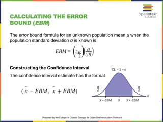
SlideShare a Scribd company logo
INTRODUCTORY STATISTICS
Chapter 8 Confidence Intervals
Prepared by the College of Coastal Georgia for OpenStax Introductory Statistics
CHAPTER 8: CONFIDENCE
INTERVALS
8.1 A Single Population Mean using the Normal Distribution
8.2 A Single Population Mean using the Student t Distribution
8.3 A Population Proportion
Prepared by the College of Coastal Georgia for OpenStax Introductory Statistics
CHAPTER OBJECTIVES
By the end of this chapter, the student should be able to:
• Calculate and interpret confidence intervals for estimating a
population mean and a population proportion.
• Interpret the Student's t probability distribution as the sample size
changes.
• Discriminate between problems applying the normal and the
Student's t distributions.
• Calculate the sample size required to estimate a population mean
and a population proportion given a desired confidence level and
margin of error.
Prepared by the College of Coastal Georgia for OpenStax Introductory Statistics
INTRODUCTION
We use sample data to make generalizations about an unknown
population. This part of statistics is called inferential statistics. The
sample data help us to make an estimate of a population
parameter.
• Suppose you were trying to determine the mean rent of a two-
bedroom apartment in your town. You might look in the classified
section of the newspaper, write down several rents listed, and
average them together. You would have obtained a point estimate
of the true mean.
• We realize that the point estimate is most likely not the exact value
of the population parameter, but close to it. After calculating point
estimates, we construct interval estimates, called confidence
intervals.
Prepared by the College of Coastal Georgia for OpenStax Introductory Statistics
POINT ESTIMATE
In this chapter, you will learn to construct and interpret confidence
intervals. You will also learn a new distribution, the Student's-t, and how it
is used with these intervals. Throughout the chapter, it is important to keep
in mind that the confidence interval is a random variable. It is the
population parameter that is fixed.
• If you worked in the marketing department of an entertainment
company, you might be interested in the mean number of songs a
consumer downloads a month from iTunes. If so, you could conduct a
survey and calculate the sample mean, x, and the sample standard
deviation, s. You would use x to estimate the population mean and s
to estimate the population standard deviation. The sample mean, x, is
the point estimate for the population mean, μ. The sample standard
deviation, s, is the point estimate for the population standard
deviation, σ.
• Each of x and s is called a statistic.
Prepared by the College of Coastal Georgia for OpenStax Introductory Statistics
CONFIDENCE INTERVAL EXAMPLE
A confidence interval is another type of estimate but, instead of being just one
number, it is an interval of numbers. The interval of numbers is a range of values
calculated from a given set of sample data. The confidence interval is likely to
include an unknown population parameter.
• Suppose, for the iTunes example, we do not know the population mean μ, but
we do know that the population standard deviation is σ = 1 and our sample
size is 100. Then, by the central limit theorem, the standard deviation for the
sample mean is
• The empirical rule, which applies to bell-shaped distributions, says that in
approximately 95% of the samples, the sample mean, x, will be within two
standard deviations of the population mean μ. For our iTunes example, two
standard deviations is (2)(0.1) = 0.2. The sample mean x is likely to be within
0.2 units of μ.
Prepared by the College of Coastal Georgia for OpenStax Introductory Statistics
ITUNES EXAMPLE CONTINUED
• Because x is within 0.2 units of μ, which is unknown, then μ is
likely to be within 0.2 units of x in 95% of the samples.
• The population mean μ is contained in an interval whose lower
number is calculated by taking the sample mean and subtracting
two standard deviations (2)(0.1) and whose upper number is
calculated by taking the sample mean and adding two standard
deviations. In other words, μ is between x − 0.2 and x + 0.2 in 95%
of all the samples.
• For the iTunes example, suppose that a sample produced a
sample mean x = 2 . Then the unknown population mean μ is
between
We say that we are 95% confident that the unknown population mean
number of songs downloaded from iTunes per month is between 1.8
and 2.2. The 95% confidence interval is (1.8, 2.2).
Prepared by the College of Coastal Georgia for OpenStax Introductory Statistics
INTERPRETATION OF THE
CONFIDENCE INTERVAL
• The 95% confidence interval implies two possibilities. Either the
interval (1.8, 2.2) contains the true mean μ or our sample produced an
x that is not within 0.2 units of the true mean μ. The second possibility
happens for only 5% of all the samples (95–100%).
• Remember that a confidence interval is created for an unknown
population parameter like the population mean, μ.
Confidence intervals for some parameters have the form:
(point estimate – margin of error, point estimate + margin of error)
• The margin of error depends on the confidence level or percentage of
confidence and the standard error of the mean.
• When you read newspapers and journals, some reports will use the
phrase "margin of error." Other reports will not use that phrase, but
include a confidence interval as the point estimate plus or minus the
margin of error. These are two ways of expressing the same concept.
Prepared by the College of Coastal Georgia for OpenStax Introductory Statistics
8.1 A SINGLE POPULATION MEAN
USING THE NORMAL DISTRIBUTION
Calculating the Confidence Interval
To construct a confidence interval for a single unknown population mean
μ, where the population standard deviation is known, we need x as an
estimate for μ and we need the margin of error. Here, the margin of error
(EBM) is called the error bound for a population mean (abbreviated
EBM). The sample mean x is the point estimate of the unknown
population mean μ.
The confidence interval estimate will have the form:
(point estimate - error bound, point estimate + error bound) or, in symbols,
Prepared by the College of Coastal Georgia for OpenStax Introductory Statistics
MARGIN OF ERROR AND
CONFIDENCE LEVEL
The margin of error (EBM) depends on the confidence level
(abbreviated CL). The confidence level is often considered the
probability that the calculated confidence interval estimate will contain
the true population parameter. However, it is more accurate to state
that the confidence level is the percent of confidence intervals that
contain the true population parameter when repeated samples are
taken. Most often, it is the choice of the person constructing the
confidence interval to choose a confidence level of 90% or higher
because that person wants to be reasonably certain of his or her
conclusions.
There is another probability called alpha (α). α is related to the
confidence level, CL. α is the probability that the interval does not
contain the unknown population parameter. Mathematically, α + CL = 1.
Prepared by the College of Coastal Georgia for OpenStax Introductory Statistics
CALCULATING THE CONFIDENCE
INTERVAL
To construct a confidence interval estimate for an unknown population
mean, we need data from a random sample. The steps to construct
and interpret the confidence interval are:
• Calculate the sample mean x from the sample data. Remember, in
this section we already know the population standard deviation σ.
• Find the z-score that corresponds to the confidence level.
• Calculate the error bound EBM.
• Construct the confidence interval.
• Write a sentence that interprets the estimate in the context of the
situation in the problem. (Explain what the confidence interval
means, in the words of the problem.)
Prepared by the College of Coastal Georgia for OpenStax Introductory Statistics
FINDING THE Z-SCORE FOR THE
STATED CONFIDENCE LEVEL
When we know the population standard deviation σ, we use a standard
normal distribution to calculate the error bound EBM and construct the
confidence interval. We need to find the value of z that puts an area equal
to the confidence level (in decimal form) in the middle of the standard
normal distribution Z ~ N(0, 1).
• The confidence level, CL, is the area in the middle of the standard normal
distribution. CL = 1 – α, so α is the area that is split equally between the
two tails. Each of the tails contains an area equal to α/2
• The z-score that has an area to the right of α/2 is denoted by zα/2.
• For example, when CL = 0.95, α = 0.05 and α/2= 0.025; we write zα/2=
z0.025.
• The area to the right of z0.025 is 0.025 and the area to the left of z0.025 is 1 –
0.025 = 0.975.
• zα/2= z0.025 = 1.96, using a calculator, computer or a standard normal
probability table.
• Calculator: invNorm(0.975, 0, 1) = 1.96
Prepared by the College of Coastal Georgia for OpenStax Introductory Statistics
CALCULATING THE ERROR
BOUND (EBM)
The error bound formula for an unknown population mean μ when the
population standard deviation σ is known is
Constructing the Confidence Interval
The confidence interval estimate has the format
Prepared by the College of Coastal Georgia for OpenStax Introductory Statistics
EXAMPLE 8.2
Suppose scores on exams in statistics are normally distributed with an
unknown population mean and a population standard deviation of three
points. A random sample of 36 scores is taken and gives a sample
mean (sample mean score) of 68. Find a confidence interval estimate
for the population mean exam score (the mean score on all exams).
Find a 90% confidence interval for the true (population) mean of
statistics exam scores.
Prepared by the College of Coastal Georgia for OpenStax Introductory Statistics
Interpretation
We estimate with 90% confidence that the true population mean exam score for all
statistics students is between 67.18 and 68.82.
Explanation of 90% Confidence Level
Ninety percent of all confidence intervals constructed in this way contain the true mean
statistics exam score. For example, if we constructed 100 of these confidence intervals,
we would expect 90 of them to contain the true population mean exam score.
Prepared by the College of Coastal Georgia for OpenStax Introductory Statistics
CALCULATING THE SAMPLE SIZE
N
If researchers desire a specific margin of error, then they can use the error
bound formula to calculate the required sample size.
The error bound formula for a population mean when the population
standard deviation is known is
The formula for sample size is , found by solving the error
bound formula for n.
In this formula, z is zα/2, corresponding to the desired confidence level. A
researcher planning a study who wants a specified confidence level and
error bound can use this formula to calculate the size of the sample
needed for the study.
Prepared by the College of Coastal Georgia for OpenStax Introductory Statistics
EXAMPLE 8.7
Prepared by the College of Coastal Georgia for OpenStax Introductory Statistics
8.2 A SINGLE POPULATION MEAN
USING THE STUDENT T
DISTRIBUTION
In practice, we rarely know the population standard deviation. In the
past, when the sample size was large, this did not present a problem to
statisticians. They used the sample standard deviation s as an estimate for
σ and proceeded as before to calculate a confidence interval with close
enough results. However, statisticians ran into problems when the sample
size was small. A small sample size caused inaccuracies in the confidence
interval.
• William S. Goset (1876–1937) of the Guinness brewery in Dublin,
Ireland ran into this problem. His experiments with hops and barley
produced very few samples. Just replacing σ with s did not produce
accurate results when he tried to calculate a confidence interval. He
realized that he could not use a normal distribution for the calculation;
he found that the actual distribution depends on the sample size. This
problem led him to "discover" what is called the Student's t-
distribution. The name comes from the fact that Gosset wrote under
the pen name "Student.“
Prepared by the College of Coastal Georgia for OpenStax Introductory Statistics
STUDENT T DISTRIBUTION
• Up until the mid-1970s, some statisticians used the normal distribution
approximation for large sample sizes and only used the Student's t-distribution
only for sample sizes of at most 30. With graphing calculators and computers,
the practice now is to use the Student's t-distribution whenever s is used as an
estimate for σ.
• If you draw a simple random sample of size n from a population that has an
approximately a normal distribution with mean μ and unknown population
standard deviation σ and calculate the t-score
• then the t-scores follow a Student's t-distribution with n – 1 degrees of
freedom. The t-score has the same interpretation as the z-score. It measures
how far x is from its mean μ. For each sample size n, there is a different
Student's t-distribution.
Prepared by the College of Coastal Georgia for OpenStax Introductory Statistics
PROPERTIES OF THE STUDENT'S
T-DISTRIBUTION
• The graph for the Student's t-distribution is similar to the standard normal
curve.
• The mean for the Student's t-distribution is zero and the distribution is
symmetric about zero.
• The Student's t-distribution has more probability in its tails than the standard
normal distribution because the spread of the t-distribution is greater than the
spread of the standard normal. So the graph of the Student's t-distribution will
be thicker in the tails and shorter in the center than the graph of the standard
normal distribution.
• The exact shape of the Student's t-distribution depends on the degrees of
freedom. As the degrees of freedom increases, the graph of Student's t-
distribution becomes more like the graph of the standard normal distribution.
• The underlying population of individual observations is assumed to be
normally distributed with unknown population mean μ and unknown population
standard deviation σ. The size of the underlying population is generally not
relevant unless it is very small. If it is bell shaped (normal) then the assumption
is met and doesn't need discussion. Random sampling is assumed, but that is
a completely separate assumption from normality.
Prepared by the College of Coastal Georgia for OpenStax Introductory Statistics
EXAMPLE 8.9
Prepared by the College of Coastal Georgia for OpenStax Introductory Statistics
EXAMPLE 8.9
SOLUTION (STEP-BY-STEP)
Prepared by the College of Coastal Georgia for OpenStax Introductory Statistics
EXAMPLE 8.9
SOLUTION (CALCULATOR)
Prepared by the College of Coastal Georgia for OpenStax Introductory Statistics
8.3 | A POPULATION PROPORTION
Example
• During an election year, we see articles in the newspaper that state
confidence intervals in terms of proportions or percentages. For
example, a poll for a particular candidate running for president
might show that the candidate has 40% of the vote within three
percentage points (if the sample is large enough). Often, election
polls are calculated with 95% confidence, so, the pollsters would
be 95% confident that the true proportion of voters who favored the
candidate would be between 0.37 and 0.43: (0.40 – 0.03,0.40 +
0.03).
The procedure to find the confidence interval, the sample size, the
error bound, and the confidence level for a proportion is similar to
that for the population mean, but the formulas are different.
Prepared by the College of Coastal Georgia for OpenStax Introductory Statistics
POPULATION PROPORTION
PROBLEM
How do you know you are dealing with a proportion problem?
First, the underlying distribution is a binomial distribution. (There is
no mention of a mean or average.) If X is a binomial random variable,
then X ~ B(n, p) where n is the number of trials and p is the probability
of a success. To form a proportion, take X, the random variable for the
number of successes and divide it by n, the number of trials (or the
sample size). The random variable P′ (read "P prime") is that
proportion,
(Sometimes the random variable is denoted as , read "P hat".)
Prepared by the College of Coastal Georgia for OpenStax Introductory Statistics
FROM BINOMIAL TO NORMAL
When n is large and p is not close to zero or one, we can use the
normal distribution to approximate the binomial.
If we divide the random variable, the mean, and the standard deviation
by n, we get a normal distribution of proportions with P′, called the
estimated proportion, as the random variable. (Recall that a proportion
as the number of successes divided by n.)
Prepared by the College of Coastal Georgia for OpenStax Introductory Statistics
FROM BINOMIAL TO NORMAL
(CONTINUED)
Using algebra to simplify :
P′ follows a normal distribution for proportions:
Prepared by the College of Coastal Georgia for OpenStax Introductory Statistics
CONFIDENCE INTERVAL FOR
PROPORTIONS
The confidence interval has the form (p′ – EBP, p′ + EBP). EBP is error
bound for the proportion.
p′ = x/n
p′ = the estimated proportion of successes (p′ is a point estimate for
p, the true proportion.)
x = the number of successes
n = the size of the sample
The error bound for a proportion is
Prepared by the College of Coastal Georgia for OpenStax Introductory Statistics
ERROR BOUND FORMULA AND
STANDARD DEVIATION
• This formula is similar to the error bound formula for a mean, except
that the "appropriate standard deviation" is different. For a mean,
when the population standard deviation is known, the appropriate
standard deviation that we use is
• For a proportion, the appropriate standard deviation is
• However, in the error bound formula, we use as the standard
deviation, instead of .
• In the error bound formula, the sample proportions p′ and q′ are
estimates of the unknown population proportions p and q. The
estimated proportions p′ and q′ are used because p and q are not
known. The sample proportions p′ and q′ are calculated from the data:
p′ is the estimated proportion of successes, and q′ is the estimated
proportion of failures.
Prepared by the College of Coastal Georgia for OpenStax Introductory Statistics
SUCCESS AND FAILURE
CONDITION
The confidence interval can be used only if the number of
successes np′ and the number of failures nq′ are both greater
than five.
Prepared by the College of Coastal Georgia for OpenStax Introductory Statistics
EXAMPLE 8.11
For a class project, a political science student at a large university
wants to estimate the percent of students who are registered voters.
He surveys 500 students and finds that 300 are registered voters.
Compute a 90% confidence interval for the true percent of students
who are registered voters, and interpret the confidence interval.
Solution 8.11
• The first solution is step-by-step (Solution A).
• The second solution uses a function of the TI-83, 83+, or 84
calculators (Solution B).
Prepared by the College of Coastal Georgia for OpenStax Introductory Statistics
EXAMPLE 8.1
SOLUTION B
Prepared by the College of Coastal Georgia for OpenStax Introductory Statistics
CALCULATING THE SAMPLE SIZE
N
If researchers desire a specific margin of error, then they can use the
error bound formula to calculate the required sample size.
• The error bound formula for a population proportion is
• Solving for n gives you an equation for the sample size.
Prepared by the College of Coastal Georgia for OpenStax Introductory Statistics
EXAMPLE 8.14
Suppose a mobile phone company wants to determine the current
percentage of customers aged 50+ who use text messaging on their
cell phones. How many customers aged 50+ should the company
survey in order to be 90% confident that the estimated (sample)
proportion is within three percentage points of the true population
proportion of customers aged 50+ who use text messaging on their cell
phones.
Prepared by the College of Coastal Georgia for OpenStax Introductory Statistics

More Related Content

What's hot

Measures of Central Tendency and Dispersion
Measures of Central Tendency and DispersionMeasures of Central Tendency and Dispersion
Measures of Central Tendency and Dispersion
Pharmacy Universe
 
Normal and standard normal distribution
Normal and standard normal distributionNormal and standard normal distribution
Normal and standard normal distribution
Avjinder (Avi) Kaler
 
Normal curve
Normal curveNormal curve
Normal curve
Lori Rapp
 
Presentation on "Measure of central tendency"
Presentation on "Measure of central tendency"Presentation on "Measure of central tendency"
Presentation on "Measure of central tendency"
muhammad raza
 
Measures of central tendency
Measures of central tendencyMeasures of central tendency
Measures of central tendency
Chie Pegollo
 
Discrete probability distribution (complete)
Discrete probability distribution (complete)Discrete probability distribution (complete)
Discrete probability distribution (complete)
ISYousafzai
 
Normal distribution
Normal distributionNormal distribution
Normal distribution
SonamWadhwa3
 
Normal distribution
Normal distributionNormal distribution
Normal distribution
Marjorie Rice
 
Statistics "Descriptive & Inferential"
Statistics "Descriptive & Inferential"Statistics "Descriptive & Inferential"
Statistics "Descriptive & Inferential"
Dalia El-Shafei
 
Probability Distributions
Probability DistributionsProbability Distributions
Probability Distributions
CIToolkit
 
Simple linear regression
Simple linear regressionSimple linear regression
Simple linear regression
Avjinder (Avi) Kaler
 
Descriptive statistics and graphs
Descriptive statistics and graphsDescriptive statistics and graphs
Descriptive statistics and graphs
Avjinder (Avi) Kaler
 
Correlation and Regression
Correlation and RegressionCorrelation and Regression
Correlation and Regression
Ram Kumar Shah "Struggler"
 
Measure of Dispersion in statistics
Measure of Dispersion in statisticsMeasure of Dispersion in statistics
Measure of Dispersion in statistics
Md. Mehadi Hassan Bappy
 
Addition rule and multiplication rule
Addition rule and multiplication rule  Addition rule and multiplication rule
Addition rule and multiplication rule
Long Beach City College
 

What's hot (20)

Measures of Central Tendency and Dispersion
Measures of Central Tendency and DispersionMeasures of Central Tendency and Dispersion
Measures of Central Tendency and Dispersion
 
Normal and standard normal distribution
Normal and standard normal distributionNormal and standard normal distribution
Normal and standard normal distribution
 
Confidence interval
Confidence intervalConfidence interval
Confidence interval
 
Normal curve
Normal curveNormal curve
Normal curve
 
Presentation on "Measure of central tendency"
Presentation on "Measure of central tendency"Presentation on "Measure of central tendency"
Presentation on "Measure of central tendency"
 
Probability concept and Probability distribution
Probability concept and Probability distributionProbability concept and Probability distribution
Probability concept and Probability distribution
 
Measures of central tendency
Measures of central tendencyMeasures of central tendency
Measures of central tendency
 
Discrete probability distribution (complete)
Discrete probability distribution (complete)Discrete probability distribution (complete)
Discrete probability distribution (complete)
 
Inferential Statistics
Inferential StatisticsInferential Statistics
Inferential Statistics
 
Normal distribution
Normal distributionNormal distribution
Normal distribution
 
Normal distribution
Normal distributionNormal distribution
Normal distribution
 
Statistics "Descriptive & Inferential"
Statistics "Descriptive & Inferential"Statistics "Descriptive & Inferential"
Statistics "Descriptive & Inferential"
 
Probability Distributions
Probability DistributionsProbability Distributions
Probability Distributions
 
Simple linear regression
Simple linear regressionSimple linear regression
Simple linear regression
 
Descriptive statistics and graphs
Descriptive statistics and graphsDescriptive statistics and graphs
Descriptive statistics and graphs
 
Correlation and Regression
Correlation and RegressionCorrelation and Regression
Correlation and Regression
 
Confidence Intervals
Confidence IntervalsConfidence Intervals
Confidence Intervals
 
Measure of Dispersion in statistics
Measure of Dispersion in statisticsMeasure of Dispersion in statistics
Measure of Dispersion in statistics
 
Addition rule and multiplication rule
Addition rule and multiplication rule  Addition rule and multiplication rule
Addition rule and multiplication rule
 
Estimation
EstimationEstimation
Estimation
 

Similar to Chapter 8

inferencial statistics
inferencial statisticsinferencial statistics
inferencial statistics
anjaemerry
 
Lec 5 statistical intervals
Lec 5 statistical intervalsLec 5 statistical intervals
Lec 5 statistical intervals
cairo university
 
statistical inference.pptx
statistical inference.pptxstatistical inference.pptx
statistical inference.pptx
SoujanyaLk1
 
Statistik 1 7 estimasi & ci
Statistik 1 7 estimasi & ciStatistik 1 7 estimasi & ci
Statistik 1 7 estimasi & ciSelvin Hadi
 
Estimating population mean
Estimating population meanEstimating population mean
Estimating population mean
Ronaldo Cabardo
 
Statistical inference: Estimation
Statistical inference: EstimationStatistical inference: Estimation
Statistical inference: Estimation
Parag Shah
 
Point and Interval Estimation
Point and Interval EstimationPoint and Interval Estimation
Point and Interval EstimationShubham Mehta
 
Confidence Intervals in the Life Sciences PresentationNamesS.docx
Confidence Intervals in the Life Sciences PresentationNamesS.docxConfidence Intervals in the Life Sciences PresentationNamesS.docx
Confidence Intervals in the Life Sciences PresentationNamesS.docx
maxinesmith73660
 
Chapter 8
Chapter 8Chapter 8
Chapter 8
MaryWall14
 
Statistical Analysis-Confidence Interval_Session 5.pptx
Statistical Analysis-Confidence Interval_Session 5.pptxStatistical Analysis-Confidence Interval_Session 5.pptx
Statistical Analysis-Confidence Interval_Session 5.pptx
maruco1
 
Estimation in statistics
Estimation in statisticsEstimation in statistics
Estimation in statistics
Rabea Jamal
 
Sampling
SamplingSampling
Sampling
Md Iqbal
 
Chapter 8 review
Chapter 8 reviewChapter 8 review
Chapter 8 reviewdrahkos1
 
Estimation and hypothesis
Estimation and hypothesisEstimation and hypothesis
Estimation and hypothesis
Junaid Ijaz
 
Msb12e ppt ch06
Msb12e ppt ch06Msb12e ppt ch06
Msb12e ppt ch06
Subas Nandy
 
Theory of estimation
Theory of estimationTheory of estimation
Theory of estimationTech_MX
 
2_Lecture 2_Confidence_Interval_3.pdf
2_Lecture 2_Confidence_Interval_3.pdf2_Lecture 2_Confidence_Interval_3.pdf
2_Lecture 2_Confidence_Interval_3.pdf
CHANSreyya1
 
Review & Hypothesis Testing
Review & Hypothesis TestingReview & Hypothesis Testing
Review & Hypothesis Testing
Sr Edith Bogue
 

Similar to Chapter 8 (20)

inferencial statistics
inferencial statisticsinferencial statistics
inferencial statistics
 
Lec 5 statistical intervals
Lec 5 statistical intervalsLec 5 statistical intervals
Lec 5 statistical intervals
 
statistical inference.pptx
statistical inference.pptxstatistical inference.pptx
statistical inference.pptx
 
Statistik 1 7 estimasi & ci
Statistik 1 7 estimasi & ciStatistik 1 7 estimasi & ci
Statistik 1 7 estimasi & ci
 
Estimating population mean
Estimating population meanEstimating population mean
Estimating population mean
 
Statistical inference: Estimation
Statistical inference: EstimationStatistical inference: Estimation
Statistical inference: Estimation
 
Point and Interval Estimation
Point and Interval EstimationPoint and Interval Estimation
Point and Interval Estimation
 
Confidence Intervals in the Life Sciences PresentationNamesS.docx
Confidence Intervals in the Life Sciences PresentationNamesS.docxConfidence Intervals in the Life Sciences PresentationNamesS.docx
Confidence Intervals in the Life Sciences PresentationNamesS.docx
 
Chapter 8
Chapter 8Chapter 8
Chapter 8
 
Statistical Analysis-Confidence Interval_Session 5.pptx
Statistical Analysis-Confidence Interval_Session 5.pptxStatistical Analysis-Confidence Interval_Session 5.pptx
Statistical Analysis-Confidence Interval_Session 5.pptx
 
Estimation in statistics
Estimation in statisticsEstimation in statistics
Estimation in statistics
 
Sampling
SamplingSampling
Sampling
 
Chapter 8 review
Chapter 8 reviewChapter 8 review
Chapter 8 review
 
Estimation and hypothesis
Estimation and hypothesisEstimation and hypothesis
Estimation and hypothesis
 
Msb12e ppt ch06
Msb12e ppt ch06Msb12e ppt ch06
Msb12e ppt ch06
 
Chapter 3
Chapter 3Chapter 3
Chapter 3
 
Chapter 3
Chapter 3Chapter 3
Chapter 3
 
Theory of estimation
Theory of estimationTheory of estimation
Theory of estimation
 
2_Lecture 2_Confidence_Interval_3.pdf
2_Lecture 2_Confidence_Interval_3.pdf2_Lecture 2_Confidence_Interval_3.pdf
2_Lecture 2_Confidence_Interval_3.pdf
 
Review & Hypothesis Testing
Review & Hypothesis TestingReview & Hypothesis Testing
Review & Hypothesis Testing
 

More from Tara Kissel, M.Ed

Chapter 12
Chapter 12Chapter 12
Chapter 12
Tara Kissel, M.Ed
 
Chapter 9
Chapter 9 Chapter 9
Chapter 9
Tara Kissel, M.Ed
 
Chapter 7
Chapter 7 Chapter 7
Chapter 7
Tara Kissel, M.Ed
 
Chapter 5 and Chapter 6
Chapter 5 and Chapter 6 Chapter 5 and Chapter 6
Chapter 5 and Chapter 6
Tara Kissel, M.Ed
 
Chapter 4
Chapter 4Chapter 4
Chapter 1 and 2
Chapter 1 and 2 Chapter 1 and 2
Chapter 1 and 2
Tara Kissel, M.Ed
 
Chapter 44: Enviromental Regulation
Chapter 44: Enviromental Regulation Chapter 44: Enviromental Regulation
Chapter 44: Enviromental Regulation
Tara Kissel, M.Ed
 
Chapter 43: Consumer Law
Chapter 43: Consumer Law Chapter 43: Consumer Law
Chapter 43: Consumer Law
Tara Kissel, M.Ed
 
Chapter 42: Antitrust Law
Chapter 42: Antitrust Law Chapter 42: Antitrust Law
Chapter 42: Antitrust Law
Tara Kissel, M.Ed
 
Chapter 41: Securities Regulation
Chapter 41: Securities RegulationChapter 41: Securities Regulation
Chapter 41: Securities Regulation
Tara Kissel, M.Ed
 
Chapter 40: Administrative Law
Chapter 40: Administrative LawChapter 40: Administrative Law
Chapter 40: Administrative Law
Tara Kissel, M.Ed
 
Chapter 39: Limited Liability Companies and Related Forms
Chapter 39: Limited Liability Companies and Related FormsChapter 39: Limited Liability Companies and Related Forms
Chapter 39: Limited Liability Companies and Related Forms
Tara Kissel, M.Ed
 
Chapter 38: Financial and Operational Features of Corporations
Chapter 38: Financial and Operational Features of CorporationsChapter 38: Financial and Operational Features of Corporations
Chapter 38: Financial and Operational Features of Corporations
Tara Kissel, M.Ed
 
Chapter 37: Nature of Corporations
Chapter 37: Nature of CorporationsChapter 37: Nature of Corporations
Chapter 37: Nature of Corporations
Tara Kissel, M.Ed
 
Chapter 36: Partnerships
Chapter 36: PartnershipsChapter 36: Partnerships
Chapter 36: Partnerships
Tara Kissel, M.Ed
 
Chapter 35: Forms of Business Organization
Chapter 35: Forms of Business Organization Chapter 35: Forms of Business Organization
Chapter 35: Forms of Business Organization
Tara Kissel, M.Ed
 
Chapter 34: Employment Discrimination
Chapter 34: Employment DiscriminationChapter 34: Employment Discrimination
Chapter 34: Employment Discrimination
Tara Kissel, M.Ed
 
Chapter 33: Employment and Labor Law
Chapter 33: Employment and Labor LawChapter 33: Employment and Labor Law
Chapter 33: Employment and Labor Law
Tara Kissel, M.Ed
 
Chapter 32: Agency Liability Concepts
Chapter 32: Agency Liability Concepts Chapter 32: Agency Liability Concepts
Chapter 32: Agency Liability Concepts
Tara Kissel, M.Ed
 
Chapter 31: Basic Principles of Agency
Chapter 31: Basic Principles of AgencyChapter 31: Basic Principles of Agency
Chapter 31: Basic Principles of Agency
Tara Kissel, M.Ed
 

More from Tara Kissel, M.Ed (20)

Chapter 12
Chapter 12Chapter 12
Chapter 12
 
Chapter 9
Chapter 9 Chapter 9
Chapter 9
 
Chapter 7
Chapter 7 Chapter 7
Chapter 7
 
Chapter 5 and Chapter 6
Chapter 5 and Chapter 6 Chapter 5 and Chapter 6
Chapter 5 and Chapter 6
 
Chapter 4
Chapter 4Chapter 4
Chapter 4
 
Chapter 1 and 2
Chapter 1 and 2 Chapter 1 and 2
Chapter 1 and 2
 
Chapter 44: Enviromental Regulation
Chapter 44: Enviromental Regulation Chapter 44: Enviromental Regulation
Chapter 44: Enviromental Regulation
 
Chapter 43: Consumer Law
Chapter 43: Consumer Law Chapter 43: Consumer Law
Chapter 43: Consumer Law
 
Chapter 42: Antitrust Law
Chapter 42: Antitrust Law Chapter 42: Antitrust Law
Chapter 42: Antitrust Law
 
Chapter 41: Securities Regulation
Chapter 41: Securities RegulationChapter 41: Securities Regulation
Chapter 41: Securities Regulation
 
Chapter 40: Administrative Law
Chapter 40: Administrative LawChapter 40: Administrative Law
Chapter 40: Administrative Law
 
Chapter 39: Limited Liability Companies and Related Forms
Chapter 39: Limited Liability Companies and Related FormsChapter 39: Limited Liability Companies and Related Forms
Chapter 39: Limited Liability Companies and Related Forms
 
Chapter 38: Financial and Operational Features of Corporations
Chapter 38: Financial and Operational Features of CorporationsChapter 38: Financial and Operational Features of Corporations
Chapter 38: Financial and Operational Features of Corporations
 
Chapter 37: Nature of Corporations
Chapter 37: Nature of CorporationsChapter 37: Nature of Corporations
Chapter 37: Nature of Corporations
 
Chapter 36: Partnerships
Chapter 36: PartnershipsChapter 36: Partnerships
Chapter 36: Partnerships
 
Chapter 35: Forms of Business Organization
Chapter 35: Forms of Business Organization Chapter 35: Forms of Business Organization
Chapter 35: Forms of Business Organization
 
Chapter 34: Employment Discrimination
Chapter 34: Employment DiscriminationChapter 34: Employment Discrimination
Chapter 34: Employment Discrimination
 
Chapter 33: Employment and Labor Law
Chapter 33: Employment and Labor LawChapter 33: Employment and Labor Law
Chapter 33: Employment and Labor Law
 
Chapter 32: Agency Liability Concepts
Chapter 32: Agency Liability Concepts Chapter 32: Agency Liability Concepts
Chapter 32: Agency Liability Concepts
 
Chapter 31: Basic Principles of Agency
Chapter 31: Basic Principles of AgencyChapter 31: Basic Principles of Agency
Chapter 31: Basic Principles of Agency
 

Recently uploaded

What are the main advantages of using HR recruiter services.pdf
What are the main advantages of using HR recruiter services.pdfWhat are the main advantages of using HR recruiter services.pdf
What are the main advantages of using HR recruiter services.pdf
HumanResourceDimensi1
 
RMD24 | Retail media: hoe zet je dit in als je geen AH of Unilever bent? Heid...
RMD24 | Retail media: hoe zet je dit in als je geen AH of Unilever bent? Heid...RMD24 | Retail media: hoe zet je dit in als je geen AH of Unilever bent? Heid...
RMD24 | Retail media: hoe zet je dit in als je geen AH of Unilever bent? Heid...
BBPMedia1
 
Introduction to Amazon company 111111111111
Introduction to Amazon company 111111111111Introduction to Amazon company 111111111111
Introduction to Amazon company 111111111111
zoyaansari11365
 
Buy Verified PayPal Account | Buy Google 5 Star Reviews
Buy Verified PayPal Account | Buy Google 5 Star ReviewsBuy Verified PayPal Account | Buy Google 5 Star Reviews
Buy Verified PayPal Account | Buy Google 5 Star Reviews
usawebmarket
 
RMD24 | Debunking the non-endemic revenue myth Marvin Vacquier Droop | First ...
RMD24 | Debunking the non-endemic revenue myth Marvin Vacquier Droop | First ...RMD24 | Debunking the non-endemic revenue myth Marvin Vacquier Droop | First ...
RMD24 | Debunking the non-endemic revenue myth Marvin Vacquier Droop | First ...
BBPMedia1
 
FINAL PRESENTATION.pptx12143241324134134
FINAL PRESENTATION.pptx12143241324134134FINAL PRESENTATION.pptx12143241324134134
FINAL PRESENTATION.pptx12143241324134134
LR1709MUSIC
 
20240425_ TJ Communications Credentials_compressed.pdf
20240425_ TJ Communications Credentials_compressed.pdf20240425_ TJ Communications Credentials_compressed.pdf
20240425_ TJ Communications Credentials_compressed.pdf
tjcomstrang
 
April 2024 Nostalgia Products Newsletter
April 2024 Nostalgia Products NewsletterApril 2024 Nostalgia Products Newsletter
April 2024 Nostalgia Products Newsletter
NathanBaughman3
 
ModelingMarketingStrategiesMKS.CollumbiaUniversitypdf
ModelingMarketingStrategiesMKS.CollumbiaUniversitypdfModelingMarketingStrategiesMKS.CollumbiaUniversitypdf
ModelingMarketingStrategiesMKS.CollumbiaUniversitypdf
fisherameliaisabella
 
Premium MEAN Stack Development Solutions for Modern Businesses
Premium MEAN Stack Development Solutions for Modern BusinessesPremium MEAN Stack Development Solutions for Modern Businesses
Premium MEAN Stack Development Solutions for Modern Businesses
SynapseIndia
 
CADAVER AS OUR FIRST TEACHER anatomt in your.pptx
CADAVER AS OUR FIRST TEACHER anatomt in your.pptxCADAVER AS OUR FIRST TEACHER anatomt in your.pptx
CADAVER AS OUR FIRST TEACHER anatomt in your.pptx
fakeloginn69
 
Sustainability: Balancing the Environment, Equity & Economy
Sustainability: Balancing the Environment, Equity & EconomySustainability: Balancing the Environment, Equity & Economy
Sustainability: Balancing the Environment, Equity & Economy
Operational Excellence Consulting
 
Search Disrupted Google’s Leaked Documents Rock the SEO World.pdf
Search Disrupted Google’s Leaked Documents Rock the SEO World.pdfSearch Disrupted Google’s Leaked Documents Rock the SEO World.pdf
Search Disrupted Google’s Leaked Documents Rock the SEO World.pdf
Arihant Webtech Pvt. Ltd
 
LA HUG - Video Testimonials with Chynna Morgan - June 2024
LA HUG - Video Testimonials with Chynna Morgan - June 2024LA HUG - Video Testimonials with Chynna Morgan - June 2024
LA HUG - Video Testimonials with Chynna Morgan - June 2024
Lital Barkan
 
Memorandum Of Association Constitution of Company.ppt
Memorandum Of Association Constitution of Company.pptMemorandum Of Association Constitution of Company.ppt
Memorandum Of Association Constitution of Company.ppt
seri bangash
 
一比一原版加拿大渥太华大学毕业证(uottawa毕业证书)如何办理
一比一原版加拿大渥太华大学毕业证(uottawa毕业证书)如何办理一比一原版加拿大渥太华大学毕业证(uottawa毕业证书)如何办理
一比一原版加拿大渥太华大学毕业证(uottawa毕业证书)如何办理
taqyed
 
What is the TDS Return Filing Due Date for FY 2024-25.pdf
What is the TDS Return Filing Due Date for FY 2024-25.pdfWhat is the TDS Return Filing Due Date for FY 2024-25.pdf
What is the TDS Return Filing Due Date for FY 2024-25.pdf
seoforlegalpillers
 
ikea_woodgreen_petscharity_dog-alogue_digital.pdf
ikea_woodgreen_petscharity_dog-alogue_digital.pdfikea_woodgreen_petscharity_dog-alogue_digital.pdf
ikea_woodgreen_petscharity_dog-alogue_digital.pdf
agatadrynko
 
VAT Registration Outlined In UAE: Benefits and Requirements
VAT Registration Outlined In UAE: Benefits and RequirementsVAT Registration Outlined In UAE: Benefits and Requirements
VAT Registration Outlined In UAE: Benefits and Requirements
uae taxgpt
 
The Influence of Marketing Strategy and Market Competition on Business Perfor...
The Influence of Marketing Strategy and Market Competition on Business Perfor...The Influence of Marketing Strategy and Market Competition on Business Perfor...
The Influence of Marketing Strategy and Market Competition on Business Perfor...
Adam Smith
 

Recently uploaded (20)

What are the main advantages of using HR recruiter services.pdf
What are the main advantages of using HR recruiter services.pdfWhat are the main advantages of using HR recruiter services.pdf
What are the main advantages of using HR recruiter services.pdf
 
RMD24 | Retail media: hoe zet je dit in als je geen AH of Unilever bent? Heid...
RMD24 | Retail media: hoe zet je dit in als je geen AH of Unilever bent? Heid...RMD24 | Retail media: hoe zet je dit in als je geen AH of Unilever bent? Heid...
RMD24 | Retail media: hoe zet je dit in als je geen AH of Unilever bent? Heid...
 
Introduction to Amazon company 111111111111
Introduction to Amazon company 111111111111Introduction to Amazon company 111111111111
Introduction to Amazon company 111111111111
 
Buy Verified PayPal Account | Buy Google 5 Star Reviews
Buy Verified PayPal Account | Buy Google 5 Star ReviewsBuy Verified PayPal Account | Buy Google 5 Star Reviews
Buy Verified PayPal Account | Buy Google 5 Star Reviews
 
RMD24 | Debunking the non-endemic revenue myth Marvin Vacquier Droop | First ...
RMD24 | Debunking the non-endemic revenue myth Marvin Vacquier Droop | First ...RMD24 | Debunking the non-endemic revenue myth Marvin Vacquier Droop | First ...
RMD24 | Debunking the non-endemic revenue myth Marvin Vacquier Droop | First ...
 
FINAL PRESENTATION.pptx12143241324134134
FINAL PRESENTATION.pptx12143241324134134FINAL PRESENTATION.pptx12143241324134134
FINAL PRESENTATION.pptx12143241324134134
 
20240425_ TJ Communications Credentials_compressed.pdf
20240425_ TJ Communications Credentials_compressed.pdf20240425_ TJ Communications Credentials_compressed.pdf
20240425_ TJ Communications Credentials_compressed.pdf
 
April 2024 Nostalgia Products Newsletter
April 2024 Nostalgia Products NewsletterApril 2024 Nostalgia Products Newsletter
April 2024 Nostalgia Products Newsletter
 
ModelingMarketingStrategiesMKS.CollumbiaUniversitypdf
ModelingMarketingStrategiesMKS.CollumbiaUniversitypdfModelingMarketingStrategiesMKS.CollumbiaUniversitypdf
ModelingMarketingStrategiesMKS.CollumbiaUniversitypdf
 
Premium MEAN Stack Development Solutions for Modern Businesses
Premium MEAN Stack Development Solutions for Modern BusinessesPremium MEAN Stack Development Solutions for Modern Businesses
Premium MEAN Stack Development Solutions for Modern Businesses
 
CADAVER AS OUR FIRST TEACHER anatomt in your.pptx
CADAVER AS OUR FIRST TEACHER anatomt in your.pptxCADAVER AS OUR FIRST TEACHER anatomt in your.pptx
CADAVER AS OUR FIRST TEACHER anatomt in your.pptx
 
Sustainability: Balancing the Environment, Equity & Economy
Sustainability: Balancing the Environment, Equity & EconomySustainability: Balancing the Environment, Equity & Economy
Sustainability: Balancing the Environment, Equity & Economy
 
Search Disrupted Google’s Leaked Documents Rock the SEO World.pdf
Search Disrupted Google’s Leaked Documents Rock the SEO World.pdfSearch Disrupted Google’s Leaked Documents Rock the SEO World.pdf
Search Disrupted Google’s Leaked Documents Rock the SEO World.pdf
 
LA HUG - Video Testimonials with Chynna Morgan - June 2024
LA HUG - Video Testimonials with Chynna Morgan - June 2024LA HUG - Video Testimonials with Chynna Morgan - June 2024
LA HUG - Video Testimonials with Chynna Morgan - June 2024
 
Memorandum Of Association Constitution of Company.ppt
Memorandum Of Association Constitution of Company.pptMemorandum Of Association Constitution of Company.ppt
Memorandum Of Association Constitution of Company.ppt
 
一比一原版加拿大渥太华大学毕业证(uottawa毕业证书)如何办理
一比一原版加拿大渥太华大学毕业证(uottawa毕业证书)如何办理一比一原版加拿大渥太华大学毕业证(uottawa毕业证书)如何办理
一比一原版加拿大渥太华大学毕业证(uottawa毕业证书)如何办理
 
What is the TDS Return Filing Due Date for FY 2024-25.pdf
What is the TDS Return Filing Due Date for FY 2024-25.pdfWhat is the TDS Return Filing Due Date for FY 2024-25.pdf
What is the TDS Return Filing Due Date for FY 2024-25.pdf
 
ikea_woodgreen_petscharity_dog-alogue_digital.pdf
ikea_woodgreen_petscharity_dog-alogue_digital.pdfikea_woodgreen_petscharity_dog-alogue_digital.pdf
ikea_woodgreen_petscharity_dog-alogue_digital.pdf
 
VAT Registration Outlined In UAE: Benefits and Requirements
VAT Registration Outlined In UAE: Benefits and RequirementsVAT Registration Outlined In UAE: Benefits and Requirements
VAT Registration Outlined In UAE: Benefits and Requirements
 
The Influence of Marketing Strategy and Market Competition on Business Perfor...
The Influence of Marketing Strategy and Market Competition on Business Perfor...The Influence of Marketing Strategy and Market Competition on Business Perfor...
The Influence of Marketing Strategy and Market Competition on Business Perfor...
 

Chapter 8

  • 1. INTRODUCTORY STATISTICS Chapter 8 Confidence Intervals Prepared by the College of Coastal Georgia for OpenStax Introductory Statistics
  • 2. CHAPTER 8: CONFIDENCE INTERVALS 8.1 A Single Population Mean using the Normal Distribution 8.2 A Single Population Mean using the Student t Distribution 8.3 A Population Proportion Prepared by the College of Coastal Georgia for OpenStax Introductory Statistics
  • 3. CHAPTER OBJECTIVES By the end of this chapter, the student should be able to: • Calculate and interpret confidence intervals for estimating a population mean and a population proportion. • Interpret the Student's t probability distribution as the sample size changes. • Discriminate between problems applying the normal and the Student's t distributions. • Calculate the sample size required to estimate a population mean and a population proportion given a desired confidence level and margin of error. Prepared by the College of Coastal Georgia for OpenStax Introductory Statistics
  • 4. INTRODUCTION We use sample data to make generalizations about an unknown population. This part of statistics is called inferential statistics. The sample data help us to make an estimate of a population parameter. • Suppose you were trying to determine the mean rent of a two- bedroom apartment in your town. You might look in the classified section of the newspaper, write down several rents listed, and average them together. You would have obtained a point estimate of the true mean. • We realize that the point estimate is most likely not the exact value of the population parameter, but close to it. After calculating point estimates, we construct interval estimates, called confidence intervals. Prepared by the College of Coastal Georgia for OpenStax Introductory Statistics
  • 5. POINT ESTIMATE In this chapter, you will learn to construct and interpret confidence intervals. You will also learn a new distribution, the Student's-t, and how it is used with these intervals. Throughout the chapter, it is important to keep in mind that the confidence interval is a random variable. It is the population parameter that is fixed. • If you worked in the marketing department of an entertainment company, you might be interested in the mean number of songs a consumer downloads a month from iTunes. If so, you could conduct a survey and calculate the sample mean, x, and the sample standard deviation, s. You would use x to estimate the population mean and s to estimate the population standard deviation. The sample mean, x, is the point estimate for the population mean, μ. The sample standard deviation, s, is the point estimate for the population standard deviation, σ. • Each of x and s is called a statistic. Prepared by the College of Coastal Georgia for OpenStax Introductory Statistics
  • 6. CONFIDENCE INTERVAL EXAMPLE A confidence interval is another type of estimate but, instead of being just one number, it is an interval of numbers. The interval of numbers is a range of values calculated from a given set of sample data. The confidence interval is likely to include an unknown population parameter. • Suppose, for the iTunes example, we do not know the population mean μ, but we do know that the population standard deviation is σ = 1 and our sample size is 100. Then, by the central limit theorem, the standard deviation for the sample mean is • The empirical rule, which applies to bell-shaped distributions, says that in approximately 95% of the samples, the sample mean, x, will be within two standard deviations of the population mean μ. For our iTunes example, two standard deviations is (2)(0.1) = 0.2. The sample mean x is likely to be within 0.2 units of μ. Prepared by the College of Coastal Georgia for OpenStax Introductory Statistics
  • 7. ITUNES EXAMPLE CONTINUED • Because x is within 0.2 units of μ, which is unknown, then μ is likely to be within 0.2 units of x in 95% of the samples. • The population mean μ is contained in an interval whose lower number is calculated by taking the sample mean and subtracting two standard deviations (2)(0.1) and whose upper number is calculated by taking the sample mean and adding two standard deviations. In other words, μ is between x − 0.2 and x + 0.2 in 95% of all the samples. • For the iTunes example, suppose that a sample produced a sample mean x = 2 . Then the unknown population mean μ is between We say that we are 95% confident that the unknown population mean number of songs downloaded from iTunes per month is between 1.8 and 2.2. The 95% confidence interval is (1.8, 2.2). Prepared by the College of Coastal Georgia for OpenStax Introductory Statistics
  • 8. INTERPRETATION OF THE CONFIDENCE INTERVAL • The 95% confidence interval implies two possibilities. Either the interval (1.8, 2.2) contains the true mean μ or our sample produced an x that is not within 0.2 units of the true mean μ. The second possibility happens for only 5% of all the samples (95–100%). • Remember that a confidence interval is created for an unknown population parameter like the population mean, μ. Confidence intervals for some parameters have the form: (point estimate – margin of error, point estimate + margin of error) • The margin of error depends on the confidence level or percentage of confidence and the standard error of the mean. • When you read newspapers and journals, some reports will use the phrase "margin of error." Other reports will not use that phrase, but include a confidence interval as the point estimate plus or minus the margin of error. These are two ways of expressing the same concept. Prepared by the College of Coastal Georgia for OpenStax Introductory Statistics
  • 9. 8.1 A SINGLE POPULATION MEAN USING THE NORMAL DISTRIBUTION Calculating the Confidence Interval To construct a confidence interval for a single unknown population mean μ, where the population standard deviation is known, we need x as an estimate for μ and we need the margin of error. Here, the margin of error (EBM) is called the error bound for a population mean (abbreviated EBM). The sample mean x is the point estimate of the unknown population mean μ. The confidence interval estimate will have the form: (point estimate - error bound, point estimate + error bound) or, in symbols, Prepared by the College of Coastal Georgia for OpenStax Introductory Statistics
  • 10. MARGIN OF ERROR AND CONFIDENCE LEVEL The margin of error (EBM) depends on the confidence level (abbreviated CL). The confidence level is often considered the probability that the calculated confidence interval estimate will contain the true population parameter. However, it is more accurate to state that the confidence level is the percent of confidence intervals that contain the true population parameter when repeated samples are taken. Most often, it is the choice of the person constructing the confidence interval to choose a confidence level of 90% or higher because that person wants to be reasonably certain of his or her conclusions. There is another probability called alpha (α). α is related to the confidence level, CL. α is the probability that the interval does not contain the unknown population parameter. Mathematically, α + CL = 1. Prepared by the College of Coastal Georgia for OpenStax Introductory Statistics
  • 11. CALCULATING THE CONFIDENCE INTERVAL To construct a confidence interval estimate for an unknown population mean, we need data from a random sample. The steps to construct and interpret the confidence interval are: • Calculate the sample mean x from the sample data. Remember, in this section we already know the population standard deviation σ. • Find the z-score that corresponds to the confidence level. • Calculate the error bound EBM. • Construct the confidence interval. • Write a sentence that interprets the estimate in the context of the situation in the problem. (Explain what the confidence interval means, in the words of the problem.) Prepared by the College of Coastal Georgia for OpenStax Introductory Statistics
  • 12. FINDING THE Z-SCORE FOR THE STATED CONFIDENCE LEVEL When we know the population standard deviation σ, we use a standard normal distribution to calculate the error bound EBM and construct the confidence interval. We need to find the value of z that puts an area equal to the confidence level (in decimal form) in the middle of the standard normal distribution Z ~ N(0, 1). • The confidence level, CL, is the area in the middle of the standard normal distribution. CL = 1 – α, so α is the area that is split equally between the two tails. Each of the tails contains an area equal to α/2 • The z-score that has an area to the right of α/2 is denoted by zα/2. • For example, when CL = 0.95, α = 0.05 and α/2= 0.025; we write zα/2= z0.025. • The area to the right of z0.025 is 0.025 and the area to the left of z0.025 is 1 – 0.025 = 0.975. • zα/2= z0.025 = 1.96, using a calculator, computer or a standard normal probability table. • Calculator: invNorm(0.975, 0, 1) = 1.96 Prepared by the College of Coastal Georgia for OpenStax Introductory Statistics
  • 13. CALCULATING THE ERROR BOUND (EBM) The error bound formula for an unknown population mean μ when the population standard deviation σ is known is Constructing the Confidence Interval The confidence interval estimate has the format Prepared by the College of Coastal Georgia for OpenStax Introductory Statistics
  • 14. EXAMPLE 8.2 Suppose scores on exams in statistics are normally distributed with an unknown population mean and a population standard deviation of three points. A random sample of 36 scores is taken and gives a sample mean (sample mean score) of 68. Find a confidence interval estimate for the population mean exam score (the mean score on all exams). Find a 90% confidence interval for the true (population) mean of statistics exam scores. Prepared by the College of Coastal Georgia for OpenStax Introductory Statistics
  • 15. Prepared by the College of Coastal Georgia for OpenStax Introductory Statistics
  • 16. Interpretation We estimate with 90% confidence that the true population mean exam score for all statistics students is between 67.18 and 68.82. Explanation of 90% Confidence Level Ninety percent of all confidence intervals constructed in this way contain the true mean statistics exam score. For example, if we constructed 100 of these confidence intervals, we would expect 90 of them to contain the true population mean exam score. Prepared by the College of Coastal Georgia for OpenStax Introductory Statistics
  • 17. Prepared by the College of Coastal Georgia for OpenStax Introductory Statistics
  • 18. CALCULATING THE SAMPLE SIZE N If researchers desire a specific margin of error, then they can use the error bound formula to calculate the required sample size. The error bound formula for a population mean when the population standard deviation is known is The formula for sample size is , found by solving the error bound formula for n. In this formula, z is zα/2, corresponding to the desired confidence level. A researcher planning a study who wants a specified confidence level and error bound can use this formula to calculate the size of the sample needed for the study. Prepared by the College of Coastal Georgia for OpenStax Introductory Statistics
  • 19. EXAMPLE 8.7 Prepared by the College of Coastal Georgia for OpenStax Introductory Statistics
  • 20. 8.2 A SINGLE POPULATION MEAN USING THE STUDENT T DISTRIBUTION In practice, we rarely know the population standard deviation. In the past, when the sample size was large, this did not present a problem to statisticians. They used the sample standard deviation s as an estimate for σ and proceeded as before to calculate a confidence interval with close enough results. However, statisticians ran into problems when the sample size was small. A small sample size caused inaccuracies in the confidence interval. • William S. Goset (1876–1937) of the Guinness brewery in Dublin, Ireland ran into this problem. His experiments with hops and barley produced very few samples. Just replacing σ with s did not produce accurate results when he tried to calculate a confidence interval. He realized that he could not use a normal distribution for the calculation; he found that the actual distribution depends on the sample size. This problem led him to "discover" what is called the Student's t- distribution. The name comes from the fact that Gosset wrote under the pen name "Student.“ Prepared by the College of Coastal Georgia for OpenStax Introductory Statistics
  • 21. STUDENT T DISTRIBUTION • Up until the mid-1970s, some statisticians used the normal distribution approximation for large sample sizes and only used the Student's t-distribution only for sample sizes of at most 30. With graphing calculators and computers, the practice now is to use the Student's t-distribution whenever s is used as an estimate for σ. • If you draw a simple random sample of size n from a population that has an approximately a normal distribution with mean μ and unknown population standard deviation σ and calculate the t-score • then the t-scores follow a Student's t-distribution with n – 1 degrees of freedom. The t-score has the same interpretation as the z-score. It measures how far x is from its mean μ. For each sample size n, there is a different Student's t-distribution. Prepared by the College of Coastal Georgia for OpenStax Introductory Statistics
  • 22. PROPERTIES OF THE STUDENT'S T-DISTRIBUTION • The graph for the Student's t-distribution is similar to the standard normal curve. • The mean for the Student's t-distribution is zero and the distribution is symmetric about zero. • The Student's t-distribution has more probability in its tails than the standard normal distribution because the spread of the t-distribution is greater than the spread of the standard normal. So the graph of the Student's t-distribution will be thicker in the tails and shorter in the center than the graph of the standard normal distribution. • The exact shape of the Student's t-distribution depends on the degrees of freedom. As the degrees of freedom increases, the graph of Student's t- distribution becomes more like the graph of the standard normal distribution. • The underlying population of individual observations is assumed to be normally distributed with unknown population mean μ and unknown population standard deviation σ. The size of the underlying population is generally not relevant unless it is very small. If it is bell shaped (normal) then the assumption is met and doesn't need discussion. Random sampling is assumed, but that is a completely separate assumption from normality. Prepared by the College of Coastal Georgia for OpenStax Introductory Statistics
  • 23. Prepared by the College of Coastal Georgia for OpenStax Introductory Statistics
  • 24. EXAMPLE 8.9 Prepared by the College of Coastal Georgia for OpenStax Introductory Statistics
  • 25. EXAMPLE 8.9 SOLUTION (STEP-BY-STEP) Prepared by the College of Coastal Georgia for OpenStax Introductory Statistics
  • 26. EXAMPLE 8.9 SOLUTION (CALCULATOR) Prepared by the College of Coastal Georgia for OpenStax Introductory Statistics
  • 27. 8.3 | A POPULATION PROPORTION Example • During an election year, we see articles in the newspaper that state confidence intervals in terms of proportions or percentages. For example, a poll for a particular candidate running for president might show that the candidate has 40% of the vote within three percentage points (if the sample is large enough). Often, election polls are calculated with 95% confidence, so, the pollsters would be 95% confident that the true proportion of voters who favored the candidate would be between 0.37 and 0.43: (0.40 – 0.03,0.40 + 0.03). The procedure to find the confidence interval, the sample size, the error bound, and the confidence level for a proportion is similar to that for the population mean, but the formulas are different. Prepared by the College of Coastal Georgia for OpenStax Introductory Statistics
  • 28. POPULATION PROPORTION PROBLEM How do you know you are dealing with a proportion problem? First, the underlying distribution is a binomial distribution. (There is no mention of a mean or average.) If X is a binomial random variable, then X ~ B(n, p) where n is the number of trials and p is the probability of a success. To form a proportion, take X, the random variable for the number of successes and divide it by n, the number of trials (or the sample size). The random variable P′ (read "P prime") is that proportion, (Sometimes the random variable is denoted as , read "P hat".) Prepared by the College of Coastal Georgia for OpenStax Introductory Statistics
  • 29. FROM BINOMIAL TO NORMAL When n is large and p is not close to zero or one, we can use the normal distribution to approximate the binomial. If we divide the random variable, the mean, and the standard deviation by n, we get a normal distribution of proportions with P′, called the estimated proportion, as the random variable. (Recall that a proportion as the number of successes divided by n.) Prepared by the College of Coastal Georgia for OpenStax Introductory Statistics
  • 30. FROM BINOMIAL TO NORMAL (CONTINUED) Using algebra to simplify : P′ follows a normal distribution for proportions: Prepared by the College of Coastal Georgia for OpenStax Introductory Statistics
  • 31. CONFIDENCE INTERVAL FOR PROPORTIONS The confidence interval has the form (p′ – EBP, p′ + EBP). EBP is error bound for the proportion. p′ = x/n p′ = the estimated proportion of successes (p′ is a point estimate for p, the true proportion.) x = the number of successes n = the size of the sample The error bound for a proportion is Prepared by the College of Coastal Georgia for OpenStax Introductory Statistics
  • 32. CONFIDENCE INTERVAL FOR PROPORTIONS The confidence interval has the form (p′ – EBP, p′ + EBP). EBP is error bound for the proportion. p′ = x/n p′ = the estimated proportion of successes (p′ is a point estimate for p, the true proportion.) x = the number of successes n = the size of the sample The error bound for a proportion is Prepared by the College of Coastal Georgia for OpenStax Introductory Statistics
  • 33. ERROR BOUND FORMULA AND STANDARD DEVIATION • This formula is similar to the error bound formula for a mean, except that the "appropriate standard deviation" is different. For a mean, when the population standard deviation is known, the appropriate standard deviation that we use is • For a proportion, the appropriate standard deviation is • However, in the error bound formula, we use as the standard deviation, instead of . • In the error bound formula, the sample proportions p′ and q′ are estimates of the unknown population proportions p and q. The estimated proportions p′ and q′ are used because p and q are not known. The sample proportions p′ and q′ are calculated from the data: p′ is the estimated proportion of successes, and q′ is the estimated proportion of failures. Prepared by the College of Coastal Georgia for OpenStax Introductory Statistics
  • 34. SUCCESS AND FAILURE CONDITION The confidence interval can be used only if the number of successes np′ and the number of failures nq′ are both greater than five. Prepared by the College of Coastal Georgia for OpenStax Introductory Statistics
  • 35. EXAMPLE 8.11 For a class project, a political science student at a large university wants to estimate the percent of students who are registered voters. He surveys 500 students and finds that 300 are registered voters. Compute a 90% confidence interval for the true percent of students who are registered voters, and interpret the confidence interval. Solution 8.11 • The first solution is step-by-step (Solution A). • The second solution uses a function of the TI-83, 83+, or 84 calculators (Solution B). Prepared by the College of Coastal Georgia for OpenStax Introductory Statistics
  • 36. Prepared by the College of Coastal Georgia for OpenStax Introductory Statistics
  • 37. EXAMPLE 8.1 SOLUTION B Prepared by the College of Coastal Georgia for OpenStax Introductory Statistics
  • 38. CALCULATING THE SAMPLE SIZE N If researchers desire a specific margin of error, then they can use the error bound formula to calculate the required sample size. • The error bound formula for a population proportion is • Solving for n gives you an equation for the sample size. Prepared by the College of Coastal Georgia for OpenStax Introductory Statistics
  • 39. EXAMPLE 8.14 Suppose a mobile phone company wants to determine the current percentage of customers aged 50+ who use text messaging on their cell phones. How many customers aged 50+ should the company survey in order to be 90% confident that the estimated (sample) proportion is within three percentage points of the true population proportion of customers aged 50+ who use text messaging on their cell phones. Prepared by the College of Coastal Georgia for OpenStax Introductory Statistics