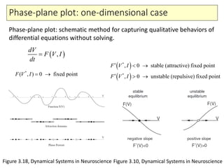
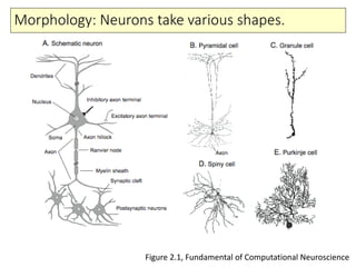
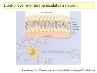
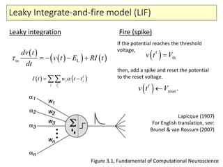
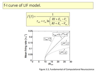
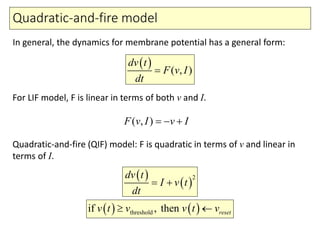
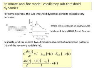
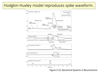
This document provides an overview of topics to be covered in a lecture on single neuron models. It will discuss: 1) The basic anatomy and physiology of neurons including their morphology and membrane properties. 2) Phenomenological models of subthreshold dynamics like the integrate-and-fire, quadratic-and-fire, and resonate-and-fire models. 3) Biophysical models of spiking mechanisms including the Hodgkin-Huxley model and its use of ion channels and master equations. 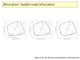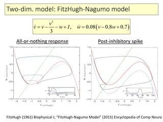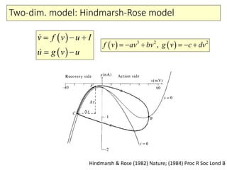4) Analysis techniques like phase plots and bifurcation analysis applied to models like FitzHugh-Nagumo and Hindmarsh-Rose. 5) Modern single neuron models such

1. SS2016 Modern Neural
Computation
Lecture 1: Single
Neurons
Hirokazu Tanaka
School of Information Science
Japan Institute of Science and Technology

2. Neuron as a computational unit of the brain.
In this lecture we will learn:
• Basic anatomy and physiology of neuron
- morphology
- membrane properties
• Phenomenological models with subthreshold dynamics
- Integrate-and-fire model, Quadratic-and-fire model,
Resonate-and-fire model
• Biophysical models with spiking mechanism
- Ion channels, master equations
- Hodgkin-Huxley model
• Phase plots and bifurcation analysis
- Saddle-node bifurcation, Andronov-Hopf bifurcation
- FitzHugh-Nagumo model, Hindmarsh-Rose model
• Modern single-neuron models
- Izhikevich model, Adaptive-exponential model

3. Neurons composed of dendrites, soma and axon.
Figure 3.1, Fundamental Neuroscience, 3rd Edition

4. Morphology: Neurons take various shapes.
Figure 2.1, Fundamental of Computational Neuroscience

5. Cortical neurons receive cortico-cortical and thalamo-
cortical inputs.
Figure 3.2, Fundamental Neuroscience, 3rd Edition
Pyramidal cell in layer II/III
Apical dendrites
Basal dendrites

6. Lipid-bilayer membrane insulates a neuron
Ruye Wang, http://fourier.eng.hmc.edu/e180/lectures/signal1/node2.html

7. Physiology: Neurons are electrically excitable.
Figure 2.2, Neuroscience 3rd Edition

8. Physiology: Neurons take various spiking patterns.
Izhikevich (2004) IEEE Neural Networks

9. Leaky Integrate-and-fire model (LIF)
( )
( )( ) ( )m L
dv t
v t E RI t
dt
τ =− − +
( ) ( )f
f
j
j j
j t
I t w t tα= −∑∑
( )f
thv t V=
( )f
reset .v t V←
Leaky integration Fire (spike)
If the potential reaches the threshold
voltage,
then, add a spike and reset the potential
to the reset voltage.
Figure 3.1, Fundamental of Computational Neuroscience
Lapicque (1907)
For English translation, see:
Brunel & van Rossum (2007)

10. Analytical solution of LIF model with constant current.
( )
( )m
dv t
v t RI
dt
τ =− +
( ) ( ) m m
0 1
t t
t
v t v e RI e RIτ τ
− −
→∞
 
= + − → 
 
 
Figure 3.2, Fundamental of Computational Neuroscience
( ) ( )
( ) const.
Lv t v t E
I t I
← −
= =
subtracting the equilibrium potential.
considering a time-invariant current.

11. f-I curve of LIF model.
Figure 3.3, Fundamental of Computational Neuroscience
( )
L r
ref m
L th
1
ln
f I
RI E V
RI E V
τ τ
=
 + −
+  
+ − 

12. Quadratic-and-fire model
( )
( )
2dv t
I v t
dt
= +
( ) ( )thresholdif , then resetv t v v t v≥ ←
( ) ( , )
dv t
F v I
dt
=
In general, the dynamics for membrane potential has a general form:
Quadratic-and-fire (QIF) model: F is quadratic in terms of v and linear in
terms of I.
For LIF model, F is linear in terms of both v and I.
( , )F v I v I=− +

13. Quadratic-and-fire model
Figure 3.35, Dynamical Systems in Neuroscience

14. Resonate-and-fire model: oscillatory sub-threshold
dynamics.
( )
( )( ) ( )
( ) ( )( )
( )
leak leak
1/2
dv t
C I g v t E w t
dt
v t vdw t
w t
dt k
=− − −
−
= −
For some neurons, the sub-threshold dynamics exhibits an oscillatory
behavior:
Resonate-and-fire model: two-dimensional model of membrane potential
(v) and the recovery variable (w).
Whole-cell recording of an olivary neuron
Hutcheon & Yarom (2000) Trends Neurosci

15. Resonate-and-fire model.
Izhikevich (2001) Neural Networks
spike
spikeno spike
no spike

16. Ion channels: Nernst equation.
Figure 6.3, Fundamental of Computational Neuroscience
[ ]
[ ]
out
ion in out
in
ion
ln
ion
RT
E E E
zF
 
≡ − =   
 
EoutEin Nernst equation
[ ]
[ ]
( )
out
out in
in
out
in
ion
ion
zF
E zFRT E E
RT
zF
E
RT
e
e
e
−
− −
−
 
 = =
 
 
 

in[ ] 140mMK+
= out[ ] 3mMK+
=
[ ]
[ ]
out
in
3
ln 61.5ln 102mV
140
K
KRT
E
F K
 
= = = −  
 
Potassium ion

17. Ion channels: Goldman-Hodgkin-Katz equation.
Figure 6.3, Fundamental of Computational Neuroscience
K Na Clout out in
m out in
K Na Clin in out
K Na Cl
ln
K Na Cl
p p pRT
V V V
F p p p
+ + −
+ + −
      + +      = − =
      + +      
Goldman-Hodgkin-Katz equation
K Na Cl: : 1.00:0.04:0.45p p p =
Permeability
For T=293K (20°C), the equilibrium potential is
m out in 62mVV V V= − =−

18. Ion-channel kinetics: voltage-dependent ion channels
:activation variablen
( )( ) ( )1n n
dn
V n V n
dt
α β= − −
Inactive Active
( )n Vα
( )n Vβ
( )activeP n=( )inactive 1P n= −
Master equation
( ) ( )n
dn
V n V n
dt
τ ∞= −
( )
( ) ( )
1
m
n n
V
V V
τ
α β
=
+
( )
( )
( ) ( )
n
n n
V
n V
V V
α
α β∞ =
+
time constant
asymptotic value
Gating equation

19. Hodgkin-Huxley model: potential and gating dynamics.
( ) ( ) ( )4 3
K K Na Na L L
dV
C g n E V g m h E V g E V I
dt
=− − − − − − +
( ) ( )n
dn
V n V n
dt
τ ∞= −
( ) ( )m
dm
V m V m
dt
τ ∞= −
( ) ( )h
dh
V h V h
dt
τ ∞= −
Membrane-potential dynamics
Gating equations
Figure 5.10, Theoretical Neuroscience

20. Hodgkin-Huxley model: activation and inactivation
variables.
( ) ( ) ( )4 3
K K Na Na L L
dV
C g n E V g m h E V g E V I
dt
=− − − − − − +
( ) ( )n
dn
V n V n
dt
τ ∞= −
( ) ( )m
dm
V m V m
dt
τ ∞= −
( ) ( )h
dh
V h V h
dt
τ ∞= −
Membrane-potential dynamics
Gating equations m: Na+ activation variable
h: Na+ inactivation variable
n: K+ activation variable
Figure 2.8, Dynamical Systems in Neuroscience
m=0
h=1
m=1
h=1
m=1
h=0

21. Hodgkin-Huxley model reproduces spike waveform.
Figure 5.10, Theoretical Neuroscience Figure 4.3, Neuroscience 3rd Edition

22. Hodgkin-Huxley model reproduces spike waveform.
Figure 2.15, Dynamical Systems in Neuroscience

23. Phase-plane plot: one-dimensional case
( ),
dV
F V I
dt
=
*
( , ) 0 fixed pointF V I= →
( )
( )
*
*
, 0 stable (attractive) fixed point
, 0 unstable (repulsive) fixed point
F V I
F V I
′ < →
′ > →
Figure 3.10, Dynamical Systems in Neuroscience
Phase-plane plot: schematic method for capturing qualitative behaviors of
differential equations without solving.
Figure 3.18, Dynamical Systems in Neuroscience

24. Bifurcation: Saddle-node bifurcation
( )
dV
F V I
dt
= +
Figure 3.25, Dynamical Systems in Neuroscience

25. Phase-plane plot: two-dimensional case
( )
( )
,
,
V F V w
w G V w
 =

=


Phase-plane plot: vector field (dV/dt, dw/dt) on the two
dimensional plane.
Figure 4.3, Dynamical Systems in Neuroscience
1, 0x y= =  0, 1x y= = 
,x x y y=− =−  ,x y y x=− =− 

26. Phase-plane plot: Nullclines
( )
( )
,
,
V F V w
w G V w
 =

=


Nullclines: the curves of F(V,w)=0 and G(V,w)=0.
Figure 4.3, Dynamical Systems in Neuroscience

27. Phase-plane plot: linear stability analysis
( )
( )
,
,
V F V w
w G V w
 =

=


Phase-plane plot: vector field (dV/dt, dw/dt) on the two
dimensional plane.
Dynamical Systems with Applications using MATLAB
Stable node Unstable node Saddle point
Unstable focus Stable focus Center

28. Phase-plane plot: Separatrix
( )
( )
,
,
V F V w
w G V w
 =

=


Phase-plane plot: vector field (dV/dt, dw/dt) on the two
dimensional plane.
Figure 4.24, Dynamical Systems in Neuroscience
Separatrix: the boundary separating two modes of behaviour in a
differential equation.

29. Bifurcation: Saddle-node bifurcation
Figure 4.26, 28, 30, Dynamical Systems in Neuroscience

30. Bifurcation: (supercritical) Andronov-Hopf bifurcation
Figure 4.26, 28, 30, Dynamical Systems in Neuroscience

31. Class I and II neurons and bifurcation type
Figure 7.3, Dynamical Systems in Neuroscience
Class I: Continuous F-I curve, Saddle-node bifurcation
Class II: Discontinuous F-I curve, Andronov-Hopf bifurcation

32. Two-dim. model: FitzHugh-Nagumo model
( )
3
3
0.08 0.8 0.7
v
v v w I
w v w
= − − +
= − +


FitzHugh (1961) Biophysical J; “FitzHugh-Nagumo Model” (2015) Encyclopedia of Comp Neuro
stable unstable
*
I I< *
I I<

33. Two-dim. model: FitzHugh-Nagumo model
( )
3
, 0.08 0.8 0.7
3
v
v v w I w v w= − − + = − + 
FitzHugh (1961) Biophysical J; “FitzHugh-Nagumo Model” (2015) Encyclopedia of Comp Neuro
All-or-nothing response Post-inhibitory spike

34. Two-dim. model: Hindmarsh-Rose model
( )
( )
v f v u I
u g v u
= − +
= −


( ) ( )3 2 2
,f v av bv g v c dv=− + =− +
Hindmarsh & Rose (1982) Nature; (1984) Proc R Soc Lond B

35. Izhikevich model: quadratic and linear nullclines.
thresholdif 1, then and .v v v c u u d≥ = ← ← +
Quadratic v-nullcline and linear u-nullcline can describe both saddle-node
and Andronov-Hopf bifurcations.
Figure 5.23, Dynamical Systems in Neuroscience
( )
2
v v u I
u a bv u
= − +
= −



36. Izhikevich model reproduces various spiking patterns.
( )
( )
2
0.04 5 140v v v u I t
u a bv u
= + + − +
= −


thresholdif 30, then and .v v v c u u d≥= ← ← +
Izhikevich (2003) IEEE Trans Neural Networks

37. Izhikevich model reproduces various spiking patterns.
Izhikevich (2003) IEEE Trans Neural Networks

38. Adaptive-exponential model
( ) ( )
( )
T
T
V V
m L T L T
w L
dV
C g V V g e w I t
dt
dw
a V E w
dt
τ
−
∆
=− − + ∆ − +
= − −
Brette & Gerstner (2005) J Neurophysiol
The adaptive-exponential model are popular to neurophysiologists
because …
- It has a form similar to conventional two-dimensional models
- Its parameters are physiologically interpretable.

39. What we left out: Neuron morphology (shape) does
influence physiology (function)!
Mainen & Sejnowski (199) Nature
250 μm
100 ms
25 mV

40. What we left out: Neuron morphology (shape) does
influence physiology (function)!
Branco et al. (2010) Science

41. Cable equation describes spike propagation.
“Cable Equation” (2015) Encyclopedia of Computational Neuroscience

42. Rall model reduces to equivalent cylinder model.
“Equivalent Cylinder Model” (2015) Encyclopedia of Computational Neuroscience
With a set of assumptions about the morphological and electrical properties of
dendrites, the complex branching structure of a dendritic tree can be reduced to
a simple conductive cylinder.
2 2
3 3
1 2
2
3
0
GR
d d
d
+
=
If GR=1, then the cylinders 1 and 2
can be reduced to a single cylinder.

43. Conclusions
- Neurons have a wide range of morphology (shapes) and
physiology (functions).
- Many fundamental properties of subthreshold dynamics
and spiking patterns can be captured by low-dimensional
models.
- Models vary in their complexities: from a simple LIF
model (just integrating and thresholding) to biophysically
detailed Hodgkin-Huxley model.
- Phase-plane and bifurcation analyses are the powerful
tool for understanding qualitative behaviors of a
dynamical system without an explicit solution.

44. Exercise
1. Read the following paper and derive a low-dimensional
neuron model from a detailed HH-type model by
linearizing around the resting potential.
Richardson et al. (2003) “From subthreshold to firing-rate
resonance,” J Neurophysiol 89, 2538-2554.
2. Examine a qualitative behavior of the Izhikevich model
by plotting a phase portrait:
a=0.02, b=0.2, c=-65, d=6, I=14 (constant).
Then confirm your phase-plane analysis with the
matlab code provided from Izhikevich’s site:
http://www.izhikevich.org/publications/whichmod.htm
#izhikevich

45. Exercise
1. Simulate an integrate-and-fire model using the Euler
method and evaluate how accurate the solution is. The
Euler method is the simplest numerical integration
method.
Brette, R., Rudolph, M., Carnevale, T., Hines, M., Beeman, D., Bower, J. M., ...
& Zirpe, M. (2007). Simulation of networks of spiking neurons: a review of
tools and strategies. Journal of computational neuroscience, 23(3), 349-398.
2. Simulate the Izhikevich model using standard
parameters. Then plot the phase portraits in two
dimensions.
( ) ( )
( )( )
m
v t RI
v t v t
t
t
τ
− +
+
∆
=∆+

46. (0.02, 0.2, -65, 8) (0.02, 0.2, -55, 4) (0.02, 0.2, -50, 2) (0.1, 0.2, -65, 2)
(0.02, 0.25, -65, 0.05) (0.02, 0.2, -65, 0.05) (0.1, 0.26, -65, 8) (0.02, 0.25, -65, 2)

47. % params for RS neuron:
a = 0.02; b = 0.20; c = -65.; d = 8;
dt = 1/1000; % integration time step (s)
T = 50.; % total simulation time (s)
t0 = 0:dt:T; % time steps
%%
v = zeros(length(t0),1); % voltage variable
u = zeros(length(t0),1); % recovery variable
I = zeros(length(t0),1); % input current
I(t0>1000/1000) = 150;
spikes = zeros(length(t0),1); % spike timings
v(1) = -80; % initial voltage
u(1) = 0; % initial recovery
for n=1:length(t0)-1
v(n+1) = v(n) + dt*(0.04*v(n)^2+5*v(n)+140-u(n)+I(n));
% v(n+1) = v(n) + dt/2*(0.04*v(n)^2+5*v(n)+140-u(n)+I(n));
% v(n+1) = v(n+1) + dt/2*(0.04*v(n+1)^2+5*v(n+1)+140-u(n)+I(n));
u(n+1) = u(n) + dt*a*(b*v(n)-u(n));
if v(n+1)>30
v(n+1) = c;
u(n+1) = u(n+1) + d;
spikes(n+1) = 1;
end
end
figure(1); clf;
subplot(211); plot(t0, v, 'k');
subplot(212); plot(t0, u, 'k');

48. References
• Squire et al. (2008) “Fundamental Neuroscience,” Academic Press.
• Purves et al. (2004) “Neuroscience,” Sinauer Associates.
• Trappenberg (2010) “Fundamentals of Computational
Neuroscience,” Oxford University Press, Chapters 2 & 3.
• Dayan & Abbott (2000) “Theoretical Neuroscience,” MIT Press,
Chapter 5.
• Izhikevich (2007) “Dynamical Systems in Neuroscience,” MIT Press,
Chapters 3 & 4.