大規模データ解析応用事例
10. ニューラルネットワークと
深層学習1
情報工学部 知能情報工学科 田中宏和
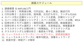
講義スケジュール
1. 講義概要 & MATLAB入門
2. 行列分解1:特異値分解、行列近似、最小二乗法、擬逆行列
3. 行列分解2:主成分分析、固有顔、次元打ち切り、ランダム化SVD
4. スパース性と圧縮センシング1:フーリエ変換、圧縮センシング
5. スパース性と圧縮センシング2:スパース回帰、スパース分類、RPCA
6. 回帰分析とモデル選択1:線形回帰、非線形回帰、数値最適化
7. 回帰分析とモデル選択2:モデル選択、交差検証法、情報量基準
8. クラスタリングと分類分析1:特徴抽出、クラスタリング法
9. クラスタリングと分類分析2:教師あり学習、分類分析
10. ニューラルネットワーク1:パーセプトロン、誤差逆伝播法
11. ニューラルネットワーク2:確率勾配法、深層ネットワーク
12. 発展学習:神経データ解析
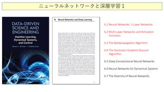
ニューラルネットワークと深層学習1
6.1 Neural Networks: 1-Layer Networks
6.2 Multi-Layer Networks and Activation
functions
6.3 The Backpropagation Algorithm
6.4 The Stochastic Gradient Descent
Algorithm
6.5 Deep Convolutional Neural Networks
6.6 Neural Networks for Dynamical Systems
6.7 The Diversity of Neural Networks
ニューラルネットワークと深層学習1
% 6.1 Neural Networks: 1-Layer Networks
CH06_SEC01_1_NN.m
% 6.2 Multi-Layer Networks
% and Activation functions
CH06_SEC01_1_NN_production.m
CH06_SEC02_1_NN.m
% 6.4 The Stochastic Gradient Descent Algorithm
CH06_SEC04_1_StochasticGradientDescent.m
% 6.5 Deep Convolutional Neural Networks
CH06_SEC05_1_DeepCNN.m
% 6.6 Neural Networks for Dynamical Systems
CH06_SEC06_1_NNLorenz.m
【本日の内容】ニューラルネットワークと深層学習1
1. ニューラルネットワーク:単層ネットワーク
- パーセプトロン(perceptron)
- パーセプトロンの限界:線形分離問題
2. ニューラルネットワーク:多層ネットワーク
- 関数近似としての教師あり学習
- 関数近似定理
3. 誤差逆伝播アルゴリズム
- 多層ニューラルネットワークの学習法1
4. 確率勾配降下アルゴリズム
- 多層ニューラルネットワークの学習法2
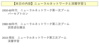
【本日の内容】ニューラルネットワークと深層学習1
1950-60年代 ニューラルネットワーク第一次ブーム
パーセプトロン
1980-90年代 ニューラルネットワーク第二次ブーム
誤差逆伝播法
2010-現在 ニューラルネットワーク第三次ブーム
深層学習
ニューラルネットワーク:単層ネットワーク
( )sgny = w x
擬逆行列を用いたパーセプトロンによる画像分類の例
% load data
load catData_w.mat;
load dogData_w.mat;
CD = [dog_wave cat_wave];
train = [dog_wave(:,1:60) cat_wave(:,1:60)];
test = [dog_wave(:,61:80) cat_wave(:,61:80)];
label = [ones(60,1); -1*ones(60,1)].';
% Pseudo-inverse solution
A_pinv=label*pinv(train);
test_labels_pinv=sign(A_pinv*test);
% LASSO solution
A_lasso = lasso(train.',label.','Lambda',0.1).';
test_labels_lasso = sign(A_lasso*test);
CH06_SEC01_1_NN_production.m 擬逆行列(Pseudo-inverse)
LASSO
パーセプトロンの幾何学
× ×
×
×
×
×
×
× ×
×
×
×
×
×
× ×
×
×
×
( )sgny = w x
1+1−
× ×
×
×
×
×
×
× ×
×
×
×
××
× ×
×
×
×
パーセプトロン学習則の収束定理(Novikov)
1+1−
×
1+1−
×
old
w
new
w
∆w
old oldnew
yη=+ +∆ =w xw w w
不正解 正解
もし学習データ(x, y)の分類が間違えた場合、重みベクトルを以下の学習則で更新する
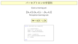
パーセプトロンの学習則
( ) ( ) ( ){ }21 1 2, , ,, , ,P Pd d dx x x
Given a training set:
Perceptron learning rule:
( )i i iydη −∆ =w x
while err>1e-4 && count<10
y = sign(w'*X)';
wnew = w + X*(d-y)/P;
wnew = wnew/norm(wnew);
count = count+1;
err = norm(w-wnew)/norm(w)
w = wnew;
end
パーセプトロンの学習則
線形分離可能な場合
パーセプトロンの学習則
線形分離不可能な場合
パーセプトロン学習則の収束定理(Novikov)
パーセプトロン学習則の収束定理
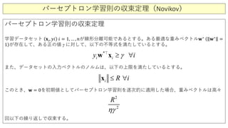
学習データセット 𝐱𝐱𝑖𝑖, 𝑦𝑦𝑦𝑦 𝑖𝑖 = 1, … , 𝑛𝑛が線形分離可能であるとする。ある最適な重みベクトル𝐰𝐰∗ (
)
𝐰𝐰∗
=
1 が存在して、ある正の値 γ に対して、以下の不等式を満たしているとする。
また、データセットの入力ベクトルのノルムは、以下の上限を満たしているとする。
このとき、𝐰𝐰 = 0を初期値としてパーセプトロン学習則を逐次的に適用した場合、重みベクトルは高々
回以下の繰り返しで収束する。
*
i i iy γ≥ ∀w x
i R i≤ ∀x
2
2
R
ηγ
パーセプトロンの記憶容量:カバーの数え上げ定理
カバーの数え上げ定理 (1965) (Cover’s Counting Theorem)
N次元空間にP個のベクトル
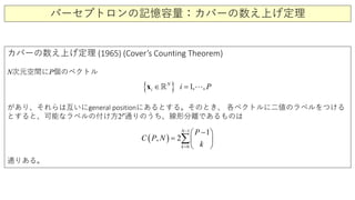
があり、それらは互いにgeneral positionにあるとする。そのとき、 各ベクトルに二値のラベルをつける
とすると、可能なラベルの付け方2P通りのうち、線形分離であるものは
通りある。
( )
1
0
1
, 2
N
k
P
C P N
k
−
=
− 
=  
 
∑
{ } 1 ,,N
i i P=∈x  
パーセプトロンの記憶容量:カバーの数え上げ定理
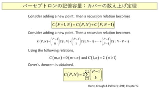
( ) ( ) ( )1, , , 1C P N C P N C P N+ = + −
Hertz, Krough & Palmer (1991) Chapter 5.
Consider adding a new point. Then a recursion relation becomes:
( ) ( ) ( ) ( )
1 1 1
, 1, 1, 1 1, 1
0 1 1
P P P
C P N C N C N C N P
P
− − −     
= + − + + − +     
−     

Consider adding a new point. Then a recursion relation becomes:
( ) ( ) ( ) ( ), 0 and 1, 2 1C m n m n C n n=< =≥
Using the following relations,
Cover’s theorem is obtained.
( )
1
0
1
, 2
N
k
P
C P N
k
−
=
− 
=  
 
∑
パーセプトロンの記憶容量:カバーの数え上げ定理
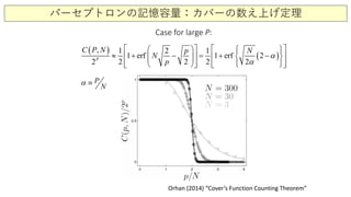
Case for large P:
Orhan (2014) “Cover’s Function Counting Theorem”
( )
( )
1 2 1
1 erf 1 erf 2
2 2 2
,
2 2P
NC pP N
N
p
α
α
       
+ − = + −               
≈
  
P
N
α ≡
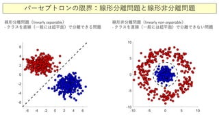
パーセプトロンの限界:線形分離問題と線形非分離問題
線形分離問題(linearly separable)
- クラスを直線(一般には超平面)で分離できる問題
線形非分離問題(linearly non-separable)
- クラスを直線(一般には超平面)で分離できない問題
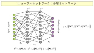
ニューラルネットワーク:多層ネットワーク
( )
( )1
1
1,f= xx W ( ) ( )
( )12
2 2 ,f=x xW ( )
( )2
3 3,f=y xW
( ) ( ) ( )
( )( )( )1
2
3 2
3 1 ,, ,f ff=y W W W x
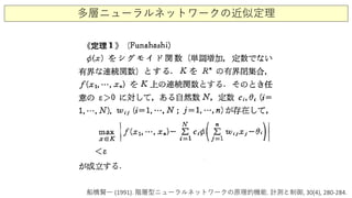
多層ニューラルネットワークの近似定理
船橋賢一 (1991). 階層型ニューラルネットワークの原理的機能. 計測と制御, 30(4), 280-284.
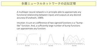
多層ニューラルネットワークの近似定理
A multilayer neural network is in principle able to approximate any
functional relationship between inputs and outputs at any desired
accuracy (Funahashi, 1989).
Intuition: A sum or a difference of two sigmoid functions is a “bump-
like” function. And, a sufficiently large number of bump functions
can approximate any function.
ワイエルシュトラスの近似定理
船橋賢一 (1991). 階層型ニューラルネットワークの原理的機能. 計測と制御, 30(4), 280-284.
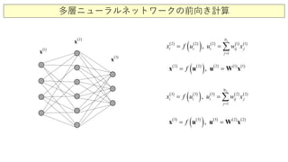
多層ニューラルネットワークの前向き計算
( )3
x
( )2
x
( )1
x
( ) ( )
( ) ( ) ( ) ( )
1
2 2 2 1 1
1
,
N
i i i ij j
j
x f u u w x
=
= = ∑
( ) ( )
( ) ( ) ( ) ( )2 2 2 1 1
,f= =x u u W x
( ) ( )
( ) ( ) ( ) ( )
2
3 3 3 2 2
1
,
N
i i i ij j
j
x f u u w x
=
= = ∑
( ) ( )
( ) ( ) ( ) ( )3 3 3 2 2
,f= =x u u W x
多層ニューラルネットワークの学習:分類問題と回帰問題
• Classification problem: to output discrete labels.
For a binary classification (i.e., 0 or 1), a cross-entropy is
often used.
• Regression problem: to output continuous values.
Sum of squared errors is often used.
ˆ:output of network, :desired outputi iy y
( ) ( ) ( )
ˆ1ˆ
: samples: samples
ˆ ˆlog 1 log 1 log 1ii
i i i i i
yy
i
ii
y y y y y y
−
− − =− + − −  ∑∏
( )
: sa p e
2
m l s
ˆi
i
iy y−∑
多層ニューラルネットワークの前向き計算
( ) ( )
( ) ( ) ( )1 1
1
n n n n
i i ij j
j
x f u f w x
− −
=
 
= =  
 
∑
( )
1
1 u
f u
e−
=
+
( )
( )
( ) ( )( )2
1 1
1
1
1
11
u
u uu
f
e
e e
u
e
f u f u
−
− −−
 
= = − = 
+ + +
′ −
Layer n-1 Layer n
( )n
ix
( )1n
jx
−
( )1n
ijw
−
( ) ( ) ( )1 1
1
n n n
i ij j
j
u w x
− −
=
= ∑
In a feedforward multilayer neural network propagates its activities
from one layer to another in one direction:
Inputs to neurons in layer n are a
summation of activities of neurons in
layer n-1:
The function f is called an activation function, and its derivative is
easy to compute:
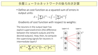
多層ニューラルネットワークの後ろ向き計算
• Define an cost function as a squared sum of errors in
output units:
Gradients of cost function with respect to weights:
( )
( ) ( )
( )
2 21 1
2 2
N N
i i i
i i
x z= − = ∆∑ ∑
Layer n-1 Layer n
( ) ( ) ( ) ( )
( ) ( )1 1
1n n n n n
i j j j ji
j
x x w− −
∆ = ∆ −∑
( )1n
j
−
∆
( )n
i∆
The neurons in the output layer has
explicit supervised errors (the difference
between the network outputs and the
desired outputs). How, then, to compute
the supervising signals for neurons in
intermediate layers?
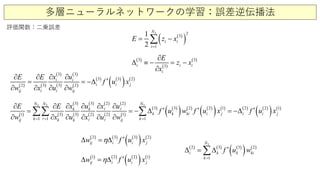
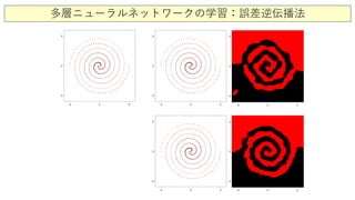
多層ニューラルネットワークの学習:誤差逆伝播法
評価関数:二乗誤差
( )
( )
3 2
3
1
1
2
i
N
i
i
E z x
=
= −∑
( ) ( )
( )
( )
( )
( )
( ) ( )
( ) ( )
3 3
3 3 2
2 3 3 2
i i
i i j
ij i i ij
x uE E
f u x
w x u w
∂ ∂∂ ∂
′∆
∂
=
∂
−
∂ ∂
( ) ( )
( )
( )
( )
( )
( )
( )
( )
( )
( ) ( )
( ) ( ) ( )
( ) ( ) ( ) ( )
( ) ( )
3 32 3 3 2 2
3 3 2 2 1 2 2 1
1 3 2
1
3 1
1 1
2
N NN
k k
k k ki i j
k
i i j
ij k k ik j
x u x uE E
f u w f u x f u x
w x u x u w==
∂ ∂ ∂ ∂∂ ∂
′ ′ ′∆ = −∆
∂ ∂ ∂
−
∂
=
∂ ∂
∑∑ ∑ 
  
( ) ( ) ( )
( ) ( )2 3 3 2
ij i i jw f u xη ′∆=∆
( ) ( ) ( )
( ) ( )1 2 2 1
ij i i jw f u xη ′∆=∆
( ) ( ) ( )
( ) ( )
3
2 3 3 2
1
N
i k k ki
k
f u w
=
′∆ = ∆∑
( )
( )
( )3 3
3i i i
i
E
z x
x
∂
∆ − −≡ =
∂
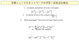
多層ニューラルネットワークの学習:誤差逆伝播法
1. Compute activations of units in all layers.
2. Compute errors in the output units, .
3. “Back-propagate” the errors to lower layers using
4. Update the weights
( )
{ } ( )
{ } ( )
{ }1
,, , ,n N
i i ix x x 
( )
{ }N
i∆
( ) ( ) ( ) ( )
( ) ( )1 1
1
n n n n n
i j j j ji
j
x x w
− −
∆ = ∆ −∑
( ) ( ) ( ) ( )
( ) ( )1 1 1
1n n n n n
ij i i i jw x x xη + + +
∆ =∆ −
多層ニューラルネットワークの学習:誤差逆伝播法
評価関数:クロスエントロピー
( )
( ) ( )
( ){ }
3
3 3
1
log 1 log 1 i
i
iii
N
E z x z x
=
= + − −∑
( ) ( )
( )
( )
( )
( )
( ) ( )
( ) ( )
3 3
3 3 2
2 3 3 2
i i
i i j
ij i i ij
x uE E
f u x
w x u w
∂ ∂∂ ∂
′∆
∂
=
∂
−
∂ ∂
( ) ( )
( )
( )
( )
( )
( )
( )
( )
( )
( ) ( )
( ) ( ) ( )
( ) ( ) ( ) ( )
( ) ( )
3 32 3 3 2 2
3 3 2 2 1 2 2 1
1 3 2
1
3 1
1 1
2
N NN
k k
k k ki i j
k
i i j
ij k k ik j
x u x uE E
f u w f u x f u x
w x u x u w==
∂ ∂ ∂ ∂∂ ∂
′ ′ ′∆ = −∆
∂ ∂ ∂
−
∂
=
∂ ∂
∑∑ ∑ 
  
( ) ( ) ( )
( ) ( )2 3 3 2
ij i i jw f u xη ′∆=∆
( ) ( ) ( )
( ) ( )1 2 2 1
ij i i jw f u xη ′∆=∆
( ) ( ) ( )
( ) ( )
3
2 3 3 2
1
N
i k k ki
k
f u w
=
′∆ = ∆∑
( )
( )
( )
( ) ( )
( )
3
3
3 3 3
1
i i
i
i i i
x zE
x x x
−∂
∆ ≡ − =
∂ −
多層ニューラルネットワークの学習:誤差逆伝播法
多層ニューラルネットワークによる画像分類の例
load catData_w.mat; load dogData_w.mat;
x=[dog_wave(:,1:40) cat_wave(:,1:40)]; % 訓練データ:イヌ画像40枚とネコ画像40枚
x2=[dog_wave(:,41:80) cat_wave(:,41:80)]; % テストデータ:イヌ画像40枚とネコ画像40枚
label=[ones(40,1) zeros(40,1);
zeros(40,1) ones(40,1)].‘; % 二つの出力ユニット(イヌ用とネコ用)
net = patternnet(2,‘trainscg’); % 入力データ ⇒ 隠れ層(2ユニット)⇒ 出力層(2ユニット)
net.layers{1}.transferFcn = ‘tansig‘; % 活性化関数 tanh
net = train(net, x, label); % ニューラルネットワークの訓練
view(net);
y = net(x); % 訓練データxに対する出力
y2= net(x2); % テストデータx2に対する出力
perf = perform(net,label,y);
classes2 = vec2ind(y);
classes3 = vec2ind(y2);
CH06_SEC02_1_NN.m
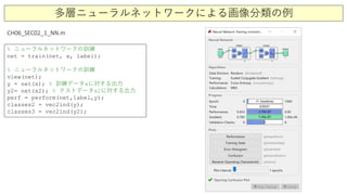
多層ニューラルネットワークによる画像分類の例
% ニューラルネットワークの訓練
net = train(net, x, label);
% ニューラルネットワークの訓練
view(net);
y = net(x); % 訓練データxに対する出力
y2= net(x2); % テストデータx2に対する出力
perf = perform(net,label,y);
classes2 = vec2ind(y);
classes3 = vec2ind(y2);
CH06_SEC02_1_NN.m
多層ニューラルネットワークによる画像分類の例
% ニューラルネットワークの訓練
net = train(net, x, label);
% ニューラルネットワークの訓練
view(net);
y = net(x); % 訓練データxに対する出力
y2= net(x2); % テストデータx2に対する出力
perf = perform(net,label,y);
classes2 = vec2ind(y);
classes3 = vec2ind(y2);
CH06_SEC02_1_NN.m
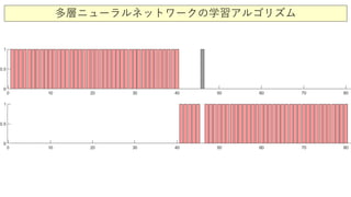
多層ニューラルネットワークによる画像分類の例
訓練データ
テストデータ
正
解
不
正
解
多層ニューラルネットワークの学習アルゴリズム
多層ニューラルネットワークの応用例(第二次ブーム)
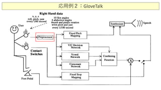
1. 英語発音学習: NetTalk (1986)
2. 手話発音学習: GloveTalk (1992)
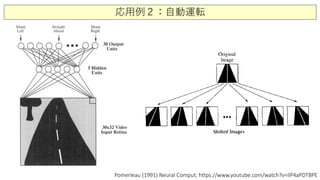
3. 自動運転: (1991)
応用例1:NetTalk
Sejnowski & Rosenberg (1987) Complex Systems; https://www.youtube.com/watch?v=gakJlr3GecE
A feedforward three-layer neural network with delay lines.
テキスト
発音
応用例1:NetTalk
Sejnowski & Rosenberg (1987) Complex Systems; https://www.youtube.com/watch?v=gakJlr3GecE
A feedforward three-layer neural network with delay lines.
DECTalk
DECtalk can be used as part of a speech generating device for those unable to speak. A notable user was Stephen Hawking, who
was unable to speak due to a combination of severe disabilities caused by ALS as well as an emergency tracheotomy.[11]
Hawking used a version of the DECtalk voice synthesizer for several years[12] and came to be associated with the unique voice of
the device. In 2011, Hawking's research assistant Sam Blackburn said Hawking still used a version of DECtalk identified on its
board as the "Calltext 5010" manufactured in 1988 by SpeechPlus, Inc.,[13] because he identified with it and had not heard a
voice he liked better. The CallText 5010 was still listed on Hawking's site as of 2015.[14] A team from Cambridge (UK) and Palo
Alto eventually emulated the workings of the CallText 5010 on a Raspberry Pi, which Hawking used from January 2018 to his
death in March of that year.[15]
The first speech synthesizer I had was almost unintelligible, but I bought a speech synthesizer which was designed for a
telephone directory service. The voice was very clear although slightly robotic. It has become my trademark, and I wouldn't
change it for a more natural voice with a British accent. I am told that children who need a computer voice want one like mine.
https://youtu.be/wn_G22hShGY
応用例2:GloveTalk
応用例2:GloveTalk
応用例2:GloveTalk
応用例2:自動運転
Pomerleau (1991) Neural Comput; https://www.youtube.com/watch?v=ilP4aPDTBPE
応用例2:自動運転
Pomerleau (1991) Neural Comput; https://www.youtube.com/watch?v=ilP4aPDTBPE
誤差逆伝播法の弱点:勾配消失問題
Hochreiter et al. (1991)
• The back-propagation algorithm works only for neural networks of
three or four layers.
• Training neural networks with many hidden layers – called “deep
neural networks”- is notoriously difficult.
( ) ( ) ( ) ( )
( ) ( )1 1
1N N N N N
j i i i ij
i
x x w− −
∆ = ∆ −∑
( ) ( ) ( ) ( )
( ) ( )
( ) ( ) ( )
( ) ( ) ( ) ( )
( ) ( )
2 1 1 1 2
1 1 1 2
1
1 1
N N N N N
k j j j jk
j
N N N N N N N
i i i ij j j jk
j i
x x w
x x w x x w
− − − − −
− − − −
∆ = ∆ −
 
= ∆ − − 
 
∑
∑ ∑
( )
( ) ( ) ( ) ( )( 1) ( 1) ( 1) ( 1) ( ) ( )
~ 1 1 1
n Nn n N N N N
x x x x x x+ + − −
∆ − × × − × − ×∆
【まとめ】ニューラルネットワークと深層学習1
1. ニューラルネットワーク:単層ネットワーク
- パーセプトロン(perceptron)
- パーセプトロンの限界:線形分離問題
2. ニューラルネットワーク:多層ネットワーク
- 関数近似としての教師あり学習
- 関数近似定理
3. 誤差逆伝播アルゴリズム
- 多層ニューラルネットワークの学習法1
4. 確率勾配降下アルゴリズム
- 多層ニューラルネットワークの学習法2

東京都市大学 データ解析入門 10 ニューラルネットワークと深層学習 1