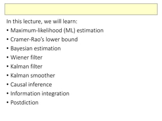
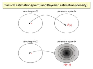
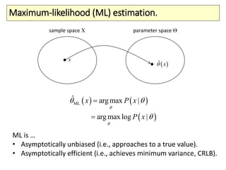
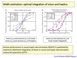
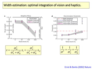
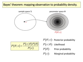
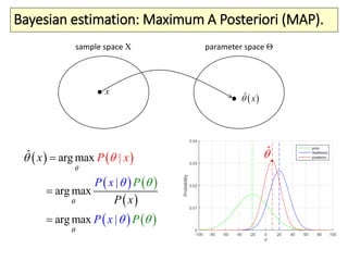
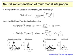
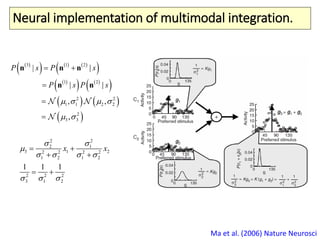
Computational Motor
Control Summer School
04: Optimal estimation
in noisy world.
Hirokazu Tanaka
School of Information Science
Japan Institute of Science and Technology
In this lecture, we will learn:
• Maximum-likelihood (ML) estimation
• Cramer-Rao’s lower bound
• Bayesian estimation
• Wiener filter
• Kalman filter
• Kalman smoother
• Causal inference
• Information integration
• Postdiction
Classical estimation (point) and Bayesian estimation (density).
sample space Χ parameter space Θ
 ˆ x
x
x
 |P x
Maximum-likelihood (ML) estimation.
sample space Χ parameter space Θ
 ˆ x
x
   
 
ML
ˆ arg max |
arg max log |
x P x
P x




 

ML is …
• Asymptotically unbiased (i.e., approaches to a true value).
• Asymptotically efficient (i.e., achieves minimum variance, CRLB).
z
Maximum-likelihood (ML) estimation.
sample space Χ parameter space Θ
 1
ˆ x
1x
2x
 2
ˆ x
 3
ˆ x
3x 0

Kullback-Leibler divergence: a distance between two density functions.
 KL ; log 0i
i
i
i
p
D q p p
q
     
 
 KL ; log 0
p x
D q p dxp x
q x
 
KL divergence for discrete variable KL divergence for continuous variable
ML as a minimization of KL divergence.
     
 
 
   
KL ; | log
|
=E log E log |
p x
D p x q x dx p x
q x
p x q x



  
      

Minimization of KL divergence
Maximization of
   KL ; |D p x q x   
 E log |q x   
   
1
1
E log | log |
N
i
iq x q x
N
 

   
KL divergence between true density p(x) and parametrized density q(x|θ):
Sampling approximation:
ML as a minimization of KL divergence.
         
    
2T
0 0
0
1
T
T
0
1
E log | log loˆ g |ˆ ˆ ˆ ˆ|
ˆ ˆ ˆ
N
i
i
q x q x E q x
N
I
      
 
    

         

 
 


 

 
   
 
2
T T
log | log |
E E
ˆ ˆ
l ˆog |ˆ
q x q x
I q x
 
 
   
 
        

 
  



 0 11ˆ ˆ, I
N
   
 
 
Sampling approximation:
ML is …
• Asymptotically unbiased (i.e., approaches to a true value).
• Asymptotically efficient (i.e., achieves minimum variance, CRLB).
Fisher information:
In the limit of large samples (infinite N), the ML estimator is unbiased and efficient.
Cramer-Rao lower bound: scalar parameter case.
Suppose a random variable 𝑋~𝑝(𝑥; 𝜃), where 𝜃 is fixed but
unknown. Assume that 𝑝(𝑥;𝜃) satisfies the “regularity” condition:
where the expectation is with respect to 𝑝(𝑥;𝜃). Then the variance
of any unbiased estimator 𝜃 satisfies
 E log | 0,p x 

 
  


 
1ˆVar
I 
   
 
   
2 2
2
log
E
|
E
| logp x p x
I
 

 
    
     
    
 

 

Fisher information:
Cramer-Rao lower bound: vector case.
Suppose a random variable 𝑋~𝑝(𝑥|𝛉), where θ is fixed but
unknown. Assume that 𝑝(𝑥|θ) satisfies the “regularity” condition:
where the expectation is with respect to 𝑝(𝑥;𝜃). Then the variance
of any unbiased estimator 𝛉 satisfies
 E log | 0,p x
 


  
θ
θ
 1ˆCov 
   θ I θ
  
     2
log | log |
E E
log |
ij
i j ji
p x p x p x 
   
   
    

  

        
θ θ
θI
Fisher information matrix:
Width estimation: optimal integration of vision and haptics.
22
H
V2 2 2 2
V V
2 2 2
V
V
H
H H
H
1 1 1
ˆ x x


   
  

 
 

Ernst & Banks (2002) Nature
     
   
 
H V
2 2
V
V
V H
2
2
2
H
H
2
, | | |
exp
2 2
exp
2
ˆ
xp x p x p x
x x
  
 
 
 


  
   
 
 
 
  
 
 
ML estimation of object width from vision and haptics:
x1: visually perceived width,
x2: haptically perceived width
σ1: visual uncertainty
σ2 : haptic uncertainty
Width estimation: optimal integration of vision and haptics.
Ernst & Banks (2002) Nature
Density functions (sensory uncertainty)
Distribution functions (human response)
By examining human forced choice, the
sensory density function can be
estimated.
Width estimation: optimal integration of vision and haptics.
Ernst & Banks (2002) Nature
mean (xV) and variance (σV
2) of vision
mean (xH) and variance (σH
2) of haptics
mean (x) and variance (σV) of
multi-modal integration
Human performance in visual-haptic discrimination (RIGHT) is predicted by
maximum-likelihood integration of those in visual and haptic discrimination
measured separately (LEFT).
Width estimation: optimal integration of vision and haptics.
Ernst & Banks (2002) Nature
22
H
1
V
H
2 2 2 2
V V H
Hx x x

   

 

V
2 2 2
H
1 1 1
  
 
Bayes’ theorem: mapping observation to probability density.
sample space Χ parameter space Θ
x
 |P x
 
   
 
|
|
P x P
P x
P x
 
 
 
 
 
 
| :
| :
:
:
P x
P x
P
P x



Posterior probability
Likelihood
Prior probability
Marginal probability
Bayesian estimation: Maximum A Posteriori (MAP).
sample space Χ parameter space Θ
 ˆ x
x
   
   
 
   
ˆ arg max
arg max
arg m
|
ax
|
|
P x
P x
P
P
P
x
P x
x




 





ˆ
Bayesian estimation: Mean minimum-squared error estimator.
sample space Χ parameter space Θ
 MMSE
ˆ x
x
   
   
2
MMSE
ˆ
2
ˆ
ˆ arg min ˆE
arg m ˆin
x x
p x d



 
   
  
  





   MMSE
ˆ x p d Ex x        
×: MAP, ×: MMSE
Motion illusion as optimal percepts.
http://www.cs.huji.ac.il/~yweiss/Rhombus/rhombus.html
Motion illusion as optimal percepts.
Weiss et al. (2002) Nature Neurosci
        
2
2
, , ,1
, | , exp
2
, , ,
, y
i i i i i i
i i x y x
I x t I xy y y
y
t I x t
P I x
x y t
t v v v v

   
     
 



 
  
   
22 2
2
1
2
, expx y x y
v
P vvv v

 
  
 
          
2
22 2
2 2
, , ,1 1
, | , ex
,
, p
,
2 2
,
y
i i i i i i
x y i i
v i
x y x
y y y
y v
x
I x t I x t I x t
P v v I x t v
y t
v v
 
   
  
  

  
   
   

Prior density: most of objects have small velocity (not moving).
Likelihood: Probability of observed image with given velocity (vx, vy).
   , , , ,x yt y t t t yI x v v I tx     Lucas-Kanade image model:
Posterior density
Motion illusion as optimal percepts.
Weiss et al. (2002) Nature Neurosci
Causal inference of sensory information.
Kording et al. (2007) PLoS One; Kayer & Shams (2015) PLoS Biol
Causal inference of sensory information.
Kording et al. (2007) PLoS One; Kayer & Shams (2015) PLoS Biol
Given visual (xV) and auditory
(xA) observations…
Q1: Do they belong to a single
object (C=1) or come from two
different objects (C=2)?
Q2: What are the most likely
positions for the visual and the
auditory objects?
Ax
Vx
Ax
Vx
Ax
Vx
Causal inference of sensory information.
Kording et al. (2007) PLoS One; Kayer & Shams (2015) PLoS Biol
 
   
       
A V
A V
A V A V
,
,
, ,
| 1 1
1|
| 1 1 | 2 2
x
x
x
P x C P C
P C x
P x C P C P x C P Cx
 
 
    
 
   
       
A V
A V
A V A V
,
,
, ,
| 2 2
2 |
| 1 1 | 2 2
x
x
x
P x C P C
P C x
P x C P C P x C P Cx
 
 
    
Bayes’ theorem:
Causal inference of sensory information.
Kording et al. (2007) PLoS One; Kayer & Shams (2015) PLoS Biol
   A A, 1 A V A, 2 A V
ˆ ˆ ˆ1| , 2 | ,C Cs s P C x x s P C x x      
   V, 1 A V V, 2V A V
ˆ ˆ ˆ1| , 2 | ,C Cs s P C x x s P C x x      
Model averaging.:
Prediction, filtering and smoothing of a dynamic system.
Prediction
Filtering
Smoothing
0 k T
 0 01: 1, ,k kz z z
 1: 1, ,k kz z z
 1: 1, ,T Tz z z
 01:k kp x z
 1:k kp x z
 1:k Tp x z
Estimation of dynamic systems: Kalman filter.
1k k k
k k k
  
 
Ax
Cx
w
z v
x
Stochastic state-space model
Problem: Given a sequence of measurements up to step k,
then estimate the conditional mean
and the conditional covariance of the state vector at step k,
 1: 1 2 ,, , , kk z z z z
| 1:
ˆ ,k k k kE   x x z
  | 1 1:
T
: : :
ˆ ˆCov E ,k k k k k k k k k k k
          
x z x x x x z
Kalman filter optimally integrates prediction and measurement.
Prediction
| 1
| 1
1| 1
T
1| 1
ˆ ˆ
k k
k
k
k
k
k k
 
 


   
x Ax
A A Q
Filtering
 
 | |
| 1
1
| | 1
ˆ ˆ ˆk k k k k k k k
k k k kk
 

  
   
x x K z Cx
I K C
 
1T T
| 1 | 1k k k k k

    K C C C RKalman gain
1| 1
1| 1
ˆk k
k k
 
 
x | 1
| 1
ˆk k
k k


x |
|
ˆk k
k k
xPrediction Filtering
kz
Kalman filter optimally integrates prediction and measurement.
1| 1
1| 1
ˆk k
k k
 
 
x | 1
| 1
ˆk k
k k


x |
|
ˆk k
k k
xPrediction Filtering
 1: 1k kp x z
 k kp z x
 1:k kp x z
 1: 1k kp x z  k kp z x  1:k kp x z
prior
likelihood
posterior
Kalman filter: Derivation.
1| 1
1| 1
ˆk k
k k
 
 
x | 1
| 1
ˆk k
k k


x |
|
ˆk k
k k
xPrediction Filtering
kz
     
   
 
1: 1 1 1 1
1 1 1 1| 1 1| 1
| 1
1
|
: 1
1
ˆ; , ; ,
ˆ; ,
kk k k k kk
k k k k k k k k
k k k k k
p d p p
d
   
    
 

 







x z x x x zx
x x Ax Q x x
x x
 1 1| 1 1| 1
ˆ; ,k k k k k    x x  | 1 | 1; ˆ ,k k k k k x x  | |; ,ˆk k k k kx x
Prediction
Filtering
 
   
 
 1: 1
1: | |
1: 1
ˆ; ,
k k k k
k k k k k k k
k k
p p
p
p


 
z x x z
x z x x
z z
Kalman filter: Derivation.
1| 1
1| 1
ˆk k
k k
 
 
x | 1
| 1
ˆk k
k k


x |
|
ˆk k
k k
xPrediction Filtering
kz
, ,
     
        
 
 
   y y
x x xy
yx
x
y
μ
y μ
x
  1 1
, 
      y yxx yy xx yyxy xyμ μx y y
  1 1
, 
     x yy xyy xx xxyx yxμ μy x x
Lemma: When a joint density function of two variables x and y are given as
then conditional probability densities are given as follows:
Kalman filter explains smooth eye pursuit movements.
Burge (2007) J Vision
 | | 1 | 1
ˆ ˆ ˆk k k k k k k k   x x K z Cx
noisy sensory feedback:
Kalman filter predicts slower
adaptation.
accurate sensory feedback:
Kalman filter predicts faster
adaptation.
Kalman filter explains smooth eye pursuit movements.
Orban de Xivry et al. (2013) J Neurosci
Kalman filter #1 for visual processing of retinal slip.
Kalman filter #2 for remembered target dynamics.
Kalman filter explains smooth eye pursuit movements.
Sinusoidal target motion Anticipatory smooth pursuit
Orban de Xivry et al. (2013) J Neurosci
Smoothing of Dynamic systems: Kalman smoother.Smoothing consists of forward and backward paths.
Filtering
Smoothing
0 k T
 1: 1, ,k kz z z
 1: 1, ,T Tz z z
 1:k kp x z
 1:k Tp x z
0 k T
Forward path  1: 1, ,k kz z z
backward path  1: 1, ,k T k T z z z
Kalman smoother algorithm: RTS smoother.
Forward path: Using the standard algorithm of Kalman filter, compute the
predicted mean and covariance,
and the filtered mean and covariance,
 1| 1| , 1,ˆ , 0,k k k k k T   x
 | |
ˆ , .0 ,,k k k k Tk x
Backward path: Then, the smoothed mean and covariance,
are solved backward in time as follows:
 | |
ˆ , .0 ,,k T k T Tk x
 
 
| | 1| 1|
| | 1| 1|
ˆ ˆ ˆ ˆk T k k k k T k k
T
k T k k k k T k k k
 
 
  
    
x x G x x
G G
 
1
| 1|
T
k k k k k

 G Awhere
Flash-lag effect explained by Kalman smoother.
http://visionlab.harvard.edu/Mem
bers/Alumni/David/flash-lag.htm
Psychophysics Extrapolation model Latency difference model Optimal smoothing model
Time
Nijhawan (1994) Whitney & Murakami (1998) Rao et al. (2001)
Rao et al. (2001) Neural Comput
Attractor neural networks for ML estimation.
   1i ij j
j
u t w o t  
Deneve et al. (1999) Nature Neurosci
 0i io a
 lim i
t
o t

Dynamics of recurrent neural network
 
 
 
2
2
1
1
1 1
i
j
i
j
u t
o t
u t

 
 
Local averaging
Divisive normalization (“winner-takes-all”)
Attractor neural networks for ML estimation.
Deneve et al. (1999) Nature Neurosci
Neural network algorithm for maximum likelihood.
  Poissoni in f s
 
 
 |
!
ii s
i
i
nf
if
s
e s
P r
n


   
 
 
1 1
|
!
|
ii
nsN fN
i
i
i
ii
f
s n
e s
P P
n
s

 
  n
 
 
   
1
1 11
log
log
|
log
|
!
N
i
N N
i i
N
i ii i
i
i
n
sP
n sP
f nfs s

  

   

  
n
Jazayeri & Movshon (2006) Nature Neurosci
Probabilistic neural responses to stimulus s:
Likelihood function:
Log likelihood function:
Neural network algorithm for maximum likelihood.
Jazayeri & Movshon (2006) Nature Neurosci
   
   
1
1 1 1
log log
log
|
!
|
N
i
N N N
i i i
i
i i i i
P P
f s r
r
r
s
f
s
s

  

   

  
r
Maximize  
1
logi i
N
i
r f s


 
1
constant
N
i
if s

under constraint
Neural implementation of multimodal integration.
Ma et al. (2006) Nature Neurosci
     
2
2
1 1 0
log | log const. const.
2
N N
i
i i i
i i
n
P s n f s s s
 
      n
   2
| ; ,s sP   n
2
21 0
1 1
,
N
i ii
N N
i ii i
n
n n
s 
 
 


 
If tuning function is Gaussian with mean si and variance σ0
2,
then, the likelihood function is also Gaussian:
where
     
2
2
0 22
00
1
, exp ,
22
i
i if ss
s s



 
  
 
 
Population activity Likelihood Population activity Likelihood
Neural implementation of multimodal integration.
Ma et al. (2006) Nature Neurosci
 
     
 
 
   
 
   
 
2
3
3 1 2
1 2
2 2
1 1 2
2
3
| |
, ,
| |
,
s s
s s
P P
P P
   
 




n n n
n n
2 2
2
3 12 2 2 2
1
1
1
2 2 2
1
2
2 2
3 2
1 1 1
x x
 

   
  
 
 
 
Summary
• Inference from noisy measurements is formulated as a
statistical inference problem.
• Statistical inference is categorized into classical point
estimation and Bayesian probability estimation.
• Human performance in psychophysical experiments
matches the predictions of optimal estimation.
• The computation of optimal inference can be
implemented by a few neural mechanisms.
References
• Ernst, M. O., & Banks, M. S. (2002). Humans integrate visual and haptic information in a statistically optimal
fashion. Nature, 415(6870), 429-433.
• Weiss, Y., Simoncelli, E. P., & Adelson, E. H. (2002). Motion illusions as optimal percepts. Nature neuroscience, 5(6),
598-604.
• Kording, K. P., & Wolpert, D. M. (2004). Bayesian integration in sensorimotor learning. Nature, 427(6971), 244-247.
• Kording, K. P., Beierholm, U., Ma, W. J., Quartz, S., Tenenbaum, J. B., & Shams, L. (2007). Causal inference in
multisensory perception.
• Kayser, C., & Shams, L. (2015). Multisensory causal inference in the brain. PLoS biology, 13(2).
• Burge, J., Ernst, M. O., & Banks, M. S. (2008). The statistical determinants of adaptation rate in human reaching.
Journal of Vision, 8(4), 20.
• de Xivry, J. J. O., Coppe, S., Blohm, G., & Lefevre, P. (2013). Kalman filtering naturally accounts for visually guided
and predictive smooth pursuit dynamics. The Journal of Neuroscience, 33(44), 17301-17313.
• Rao, R. P., Eagleman, D. M., & Sejnowski, T. J. (2001). Optimal smoothing in visual motion perception. Neural
Computation, 13(6), 1243-1253.
• Deneve, S., Latham, P. E., & Pouget, A. (1999). Reading population codes: a neural implementation of ideal
observers. Nature neuroscience, 2(8), 740-745.
• Jazayeri, M., & Movshon, J. A. (2006). Optimal representation of sensory information by neural populations. Nature
neuroscience, 9(5), 690-696.
• Ma, W. J., Beck, J. M., Latham, P. E., & Pouget, A. (2006). Bayesian inference with probabilistic population codes.
Nature neuroscience, 9(11), 1432-1438.
Exercise
• Write a Matlab code for Kalman filter and Kalman
smoothing, and examine the difference.
• Psychophysics: Smooth eye pursuit experiment using
GazeParser (http://gazeparser.sourceforge.net/).

Computational Motor Control: Optimal Estimation in Noisy World (JAIST summer course)

  • 1.
    Computational Motor Control SummerSchool 04: Optimal estimation in noisy world. Hirokazu Tanaka School of Information Science Japan Institute of Science and Technology
  • 2.
    In this lecture,we will learn: • Maximum-likelihood (ML) estimation • Cramer-Rao’s lower bound • Bayesian estimation • Wiener filter • Kalman filter • Kalman smoother • Causal inference • Information integration • Postdiction
  • 3.
    Classical estimation (point)and Bayesian estimation (density). sample space Χ parameter space Θ sample space Χ parameter space Θ  ˆ x x x  |P x
  • 4.
    Maximum-likelihood (ML) estimation. samplespace Χ parameter space Θ  ˆ x x       ML ˆ arg max | arg max log | x P x P x        ML is … • Asymptotically unbiased (i.e., approaches to a true value). • Asymptotically efficient (i.e., achieves minimum variance, CRLB).
  • 5.
    z Maximum-likelihood (ML) estimation. samplespace Χ parameter space Θ  1 ˆ x 1x 2x  2 ˆ x  3 ˆ x 3x 0 
  • 6.
    Kullback-Leibler divergence: adistance between two density functions.  KL ; log 0i i i i p D q p p q          KL ; log 0 p x D q p dxp x q x   KL divergence for discrete variable KL divergence for continuous variable
  • 7.
    ML as aminimization of KL divergence.               KL ; | log | =E log E log | p x D p x q x dx p x q x p x q x               Minimization of KL divergence Maximization of    KL ; |D p x q x     E log |q x        1 1 E log | log | N i iq x q x N        KL divergence between true density p(x) and parametrized density q(x|θ): Sampling approximation:
  • 8.
    ML as aminimization of KL divergence.                2T 0 0 0 1 T T 0 1 E log | log loˆ g |ˆ ˆ ˆ ˆ| ˆ ˆ ˆ N i i q x q x E q x N I                                            2 T T log | log | E E ˆ ˆ l ˆog |ˆ q x q x I q x                              0 11ˆ ˆ, I N         Sampling approximation: ML is … • Asymptotically unbiased (i.e., approaches to a true value). • Asymptotically efficient (i.e., achieves minimum variance, CRLB). Fisher information: In the limit of large samples (infinite N), the ML estimator is unbiased and efficient.
  • 9.
    Cramer-Rao lower bound:scalar parameter case. Suppose a random variable 𝑋~𝑝(𝑥; 𝜃), where 𝜃 is fixed but unknown. Assume that 𝑝(𝑥;𝜃) satisfies the “regularity” condition: where the expectation is with respect to 𝑝(𝑥;𝜃). Then the variance of any unbiased estimator 𝜃 satisfies  E log | 0,p x            1ˆVar I            2 2 2 log E | E | logp x p x I                            Fisher information:
  • 10.
    Cramer-Rao lower bound:vector case. Suppose a random variable 𝑋~𝑝(𝑥|𝛉), where θ is fixed but unknown. Assume that 𝑝(𝑥|θ) satisfies the “regularity” condition: where the expectation is with respect to 𝑝(𝑥;𝜃). Then the variance of any unbiased estimator 𝛉 satisfies  E log | 0,p x        θ θ  1ˆCov     θ I θ         2 log | log | E E log | ij i j ji p x p x p x                             θ θ θI Fisher information matrix:
  • 11.
    Width estimation: optimalintegration of vision and haptics. 22 H V2 2 2 2 V V 2 2 2 V V H H H H 1 1 1 ˆ x x                Ernst & Banks (2002) Nature             H V 2 2 V V V H 2 2 2 H H 2 , | | | exp 2 2 exp 2 ˆ xp x p x p x x x                                ML estimation of object width from vision and haptics: x1: visually perceived width, x2: haptically perceived width σ1: visual uncertainty σ2 : haptic uncertainty
  • 12.
    Width estimation: optimalintegration of vision and haptics. Ernst & Banks (2002) Nature Density functions (sensory uncertainty) Distribution functions (human response) By examining human forced choice, the sensory density function can be estimated.
  • 13.
    Width estimation: optimalintegration of vision and haptics. Ernst & Banks (2002) Nature mean (xV) and variance (σV 2) of vision mean (xH) and variance (σH 2) of haptics mean (x) and variance (σV) of multi-modal integration Human performance in visual-haptic discrimination (RIGHT) is predicted by maximum-likelihood integration of those in visual and haptic discrimination measured separately (LEFT).
  • 14.
    Width estimation: optimalintegration of vision and haptics. Ernst & Banks (2002) Nature 22 H 1 V H 2 2 2 2 V V H Hx x x          V 2 2 2 H 1 1 1     
  • 15.
    Bayes’ theorem: mappingobservation to probability density. sample space Χ parameter space Θ x  |P x         | | P x P P x P x             | : | : : : P x P x P P x    Posterior probability Likelihood Prior probability Marginal probability
  • 16.
    Bayesian estimation: MaximumA Posteriori (MAP). sample space Χ parameter space Θ  ˆ x x               ˆ arg max arg max arg m | ax | | P x P x P P P x P x x            ˆ
  • 17.
    Bayesian estimation: Meanminimum-squared error estimator. sample space Χ parameter space Θ  MMSE ˆ x x         2 MMSE ˆ 2 ˆ ˆ arg min ˆE arg m ˆin x x p x d                        MMSE ˆ x p d Ex x         ×: MAP, ×: MMSE
  • 18.
    Motion illusion asoptimal percepts. http://www.cs.huji.ac.il/~yweiss/Rhombus/rhombus.html
  • 19.
    Motion illusion asoptimal percepts. Weiss et al. (2002) Nature Neurosci          2 2 , , ,1 , | , exp 2 , , , , y i i i i i i i i x y x I x t I xy y y y t I x t P I x x y t t v v v v                          22 2 2 1 2 , expx y x y v P vvv v                    2 22 2 2 2 , , ,1 1 , | , ex , , p , 2 2 , y i i i i i i x y i i v i x y x y y y y v x I x t I x t I x t P v v I x t v y t v v                          Prior density: most of objects have small velocity (not moving). Likelihood: Probability of observed image with given velocity (vx, vy).    , , , ,x yt y t t t yI x v v I tx     Lucas-Kanade image model: Posterior density
  • 20.
    Motion illusion asoptimal percepts. Weiss et al. (2002) Nature Neurosci
  • 21.
    Causal inference ofsensory information. Kording et al. (2007) PLoS One; Kayer & Shams (2015) PLoS Biol
  • 22.
    Causal inference ofsensory information. Kording et al. (2007) PLoS One; Kayer & Shams (2015) PLoS Biol Given visual (xV) and auditory (xA) observations… Q1: Do they belong to a single object (C=1) or come from two different objects (C=2)? Q2: What are the most likely positions for the visual and the auditory objects? Ax Vx Ax Vx Ax Vx
  • 23.
    Causal inference ofsensory information. Kording et al. (2007) PLoS One; Kayer & Shams (2015) PLoS Biol               A V A V A V A V , , , , | 1 1 1| | 1 1 | 2 2 x x x P x C P C P C x P x C P C P x C P Cx                        A V A V A V A V , , , , | 2 2 2 | | 1 1 | 2 2 x x x P x C P C P C x P x C P C P x C P Cx          Bayes’ theorem:
  • 24.
    Causal inference ofsensory information. Kording et al. (2007) PLoS One; Kayer & Shams (2015) PLoS Biol    A A, 1 A V A, 2 A V ˆ ˆ ˆ1| , 2 | ,C Cs s P C x x s P C x x          V, 1 A V V, 2V A V ˆ ˆ ˆ1| , 2 | ,C Cs s P C x x s P C x x       Model averaging.:
  • 25.
    Prediction, filtering andsmoothing of a dynamic system. Prediction Filtering Smoothing 0 k T  0 01: 1, ,k kz z z  1: 1, ,k kz z z  1: 1, ,T Tz z z  01:k kp x z  1:k kp x z  1:k Tp x z
  • 26.
    Estimation of dynamicsystems: Kalman filter. 1k k k k k k      Ax Cx w z v x Stochastic state-space model Problem: Given a sequence of measurements up to step k, then estimate the conditional mean and the conditional covariance of the state vector at step k,  1: 1 2 ,, , , kk z z z z | 1: ˆ ,k k k kE   x x z   | 1 1: T : : : ˆ ˆCov E ,k k k k k k k k k k k            x z x x x x z
  • 27.
    Kalman filter optimallyintegrates prediction and measurement. Prediction | 1 | 1 1| 1 T 1| 1 ˆ ˆ k k k k k k k k           x Ax A A Q Filtering    | | | 1 1 | | 1 ˆ ˆ ˆk k k k k k k k k k k kk           x x K z Cx I K C   1T T | 1 | 1k k k k k      K C C C RKalman gain 1| 1 1| 1 ˆk k k k     x | 1 | 1 ˆk k k k   x | | ˆk k k k xPrediction Filtering kz
  • 28.
    Kalman filter optimallyintegrates prediction and measurement. 1| 1 1| 1 ˆk k k k     x | 1 | 1 ˆk k k k   x | | ˆk k k k xPrediction Filtering  1: 1k kp x z  k kp z x  1:k kp x z  1: 1k kp x z  k kp z x  1:k kp x z prior likelihood posterior
  • 29.
    Kalman filter: Derivation. 1|1 1| 1 ˆk k k k     x | 1 | 1 ˆk k k k   x | | ˆk k k k xPrediction Filtering kz             1: 1 1 1 1 1 1 1 1| 1 1| 1 | 1 1 | : 1 1 ˆ; , ; , ˆ; , kk k k k kk k k k k k k k k k k k k k p d p p d                      x z x x x zx x x Ax Q x x x x  1 1| 1 1| 1 ˆ; ,k k k k k    x x  | 1 | 1; ˆ ,k k k k k x x  | |; ,ˆk k k k kx x Prediction Filtering          1: 1 1: | | 1: 1 ˆ; , k k k k k k k k k k k k k p p p p     z x x z x z x x z z
  • 30.
    Kalman filter: Derivation. 1|1 1| 1 ˆk k k k     x | 1 | 1 ˆk k k k   x | | ˆk k k k xPrediction Filtering kz , ,                       y y x x xy yx x y μ y μ x   1 1 ,        y yxx yy xx yyxy xyμ μx y y   1 1 ,       x yy xyy xx xxyx yxμ μy x x Lemma: When a joint density function of two variables x and y are given as then conditional probability densities are given as follows:
  • 31.
    Kalman filter explainssmooth eye pursuit movements. Burge (2007) J Vision  | | 1 | 1 ˆ ˆ ˆk k k k k k k k   x x K z Cx noisy sensory feedback: Kalman filter predicts slower adaptation. accurate sensory feedback: Kalman filter predicts faster adaptation.
  • 32.
    Kalman filter explainssmooth eye pursuit movements. Orban de Xivry et al. (2013) J Neurosci Kalman filter #1 for visual processing of retinal slip. Kalman filter #2 for remembered target dynamics.
  • 33.
    Kalman filter explainssmooth eye pursuit movements. Sinusoidal target motion Anticipatory smooth pursuit Orban de Xivry et al. (2013) J Neurosci
  • 34.
    Smoothing of Dynamicsystems: Kalman smoother.Smoothing consists of forward and backward paths. Filtering Smoothing 0 k T  1: 1, ,k kz z z  1: 1, ,T Tz z z  1:k kp x z  1:k Tp x z 0 k T Forward path  1: 1, ,k kz z z backward path  1: 1, ,k T k T z z z
  • 35.
    Kalman smoother algorithm:RTS smoother. Forward path: Using the standard algorithm of Kalman filter, compute the predicted mean and covariance, and the filtered mean and covariance,  1| 1| , 1,ˆ , 0,k k k k k T   x  | | ˆ , .0 ,,k k k k Tk x Backward path: Then, the smoothed mean and covariance, are solved backward in time as follows:  | | ˆ , .0 ,,k T k T Tk x     | | 1| 1| | | 1| 1| ˆ ˆ ˆ ˆk T k k k k T k k T k T k k k k T k k k             x x G x x G G   1 | 1| T k k k k k   G Awhere
  • 36.
    Flash-lag effect explainedby Kalman smoother. http://visionlab.harvard.edu/Mem bers/Alumni/David/flash-lag.htm Psychophysics Extrapolation model Latency difference model Optimal smoothing model Time Nijhawan (1994) Whitney & Murakami (1998) Rao et al. (2001) Rao et al. (2001) Neural Comput
  • 37.
    Attractor neural networksfor ML estimation.    1i ij j j u t w o t   Deneve et al. (1999) Nature Neurosci  0i io a  lim i t o t  Dynamics of recurrent neural network       2 2 1 1 1 1 i j i j u t o t u t      Local averaging Divisive normalization (“winner-takes-all”)
  • 38.
    Attractor neural networksfor ML estimation. Deneve et al. (1999) Nature Neurosci
  • 39.
    Neural network algorithmfor maximum likelihood.   Poissoni in f s      | ! ii s i i nf if s e s P r n           1 1 | ! | ii nsN fN i i i ii f s n e s P P n s      n         1 1 11 log log | log | ! N i N N i i N i ii i i i n sP n sP f nfs s              n Jazayeri & Movshon (2006) Nature Neurosci Probabilistic neural responses to stimulus s: Likelihood function: Log likelihood function:
  • 40.
    Neural network algorithmfor maximum likelihood. Jazayeri & Movshon (2006) Nature Neurosci         1 1 1 1 log log log | ! | N i N N N i i i i i i i i P P f s r r r s f s s              r Maximize   1 logi i N i r f s     1 constant N i if s  under constraint
  • 41.
    Neural implementation ofmultimodal integration. Ma et al. (2006) Nature Neurosci       2 2 1 1 0 log | log const. const. 2 N N i i i i i i n P s n f s s s         n    2 | ; ,s sP   n 2 21 0 1 1 , N i ii N N i ii i n n n s          If tuning function is Gaussian with mean si and variance σ0 2, then, the likelihood function is also Gaussian: where       2 2 0 22 00 1 , exp , 22 i i if ss s s             Population activity Likelihood Population activity Likelihood
  • 42.
    Neural implementation ofmultimodal integration. Ma et al. (2006) Nature Neurosci                         2 3 3 1 2 1 2 2 2 1 1 2 2 3 | | , , | | , s s s s P P P P           n n n n n 2 2 2 3 12 2 2 2 1 1 1 2 2 2 1 2 2 2 3 2 1 1 1 x x                
  • 43.
    Summary • Inference fromnoisy measurements is formulated as a statistical inference problem. • Statistical inference is categorized into classical point estimation and Bayesian probability estimation. • Human performance in psychophysical experiments matches the predictions of optimal estimation. • The computation of optimal inference can be implemented by a few neural mechanisms.
  • 44.
    References • Ernst, M.O., & Banks, M. S. (2002). Humans integrate visual and haptic information in a statistically optimal fashion. Nature, 415(6870), 429-433. • Weiss, Y., Simoncelli, E. P., & Adelson, E. H. (2002). Motion illusions as optimal percepts. Nature neuroscience, 5(6), 598-604. • Kording, K. P., & Wolpert, D. M. (2004). Bayesian integration in sensorimotor learning. Nature, 427(6971), 244-247. • Kording, K. P., Beierholm, U., Ma, W. J., Quartz, S., Tenenbaum, J. B., & Shams, L. (2007). Causal inference in multisensory perception. • Kayser, C., & Shams, L. (2015). Multisensory causal inference in the brain. PLoS biology, 13(2). • Burge, J., Ernst, M. O., & Banks, M. S. (2008). The statistical determinants of adaptation rate in human reaching. Journal of Vision, 8(4), 20. • de Xivry, J. J. O., Coppe, S., Blohm, G., & Lefevre, P. (2013). Kalman filtering naturally accounts for visually guided and predictive smooth pursuit dynamics. The Journal of Neuroscience, 33(44), 17301-17313. • Rao, R. P., Eagleman, D. M., & Sejnowski, T. J. (2001). Optimal smoothing in visual motion perception. Neural Computation, 13(6), 1243-1253. • Deneve, S., Latham, P. E., & Pouget, A. (1999). Reading population codes: a neural implementation of ideal observers. Nature neuroscience, 2(8), 740-745. • Jazayeri, M., & Movshon, J. A. (2006). Optimal representation of sensory information by neural populations. Nature neuroscience, 9(5), 690-696. • Ma, W. J., Beck, J. M., Latham, P. E., & Pouget, A. (2006). Bayesian inference with probabilistic population codes. Nature neuroscience, 9(11), 1432-1438.
  • 45.
    Exercise • Write aMatlab code for Kalman filter and Kalman smoothing, and examine the difference. • Psychophysics: Smooth eye pursuit experiment using GazeParser (http://gazeparser.sourceforge.net/).