Download to read offline


![Allan Turing (1950)
Computing machinery and intelligence. Mind, 59, 433-460.
Is there a corresponding phenomenon [criticality] for minds, and
is there one for machines? There does seem to be one for the
human mind. The majority of them seems to be subcritical, i.e., to
correspond in this analogy to piles of subcritical size. An idea
presented to such a mind will on average give rise to less than one
idea in reply.
A smallish proportion are supercritical. An idea presented to such
a mind may give rise to a whole "theory" consisting of secondary,
tertiary and more remote ideas. (...) Adhering to this analogy we
ask, "Can a machine be made to be supercritical?"
4](https://image.slidesharecdn.com/sosckinouchi2-171216155803/75/Neuronal-self-organized-criticality-4-2048.jpg)

![Our model: Stochastic discrete time spiking
neurons (Galves & Löcherbach, 2013)
i = 1, 2, …, N neurons Xi[t] = 1 (spike)
Vi[t+1] = 0 reset if Xi[t] = 1
Vi[t+1] = μVi[t] + I + N-1 ∑j Wij Xj[t] if Xi[t] = 0
Prob( Xi[t+1] = 1 ) = Φ(Vi[t])
Φ = firing probability function
0 ≤ Φ(V) ≤ 1
7
All-to-all network](https://image.slidesharecdn.com/sosckinouchi2-171216155803/75/Neuronal-self-organized-criticality-6-2048.jpg)
![Examples of firing functions
8
1
VT VS V
r = 1
r > 1
r < 1
Φ(V) For VT < V < VS: Φ(V) = [ 𝚪(V-VT) ]r
𝚪 = Neuronal Gain](https://image.slidesharecdn.com/sosckinouchi2-171216155803/75/Neuronal-self-organized-criticality-7-2048.jpg)
![Mean field approach
Order parameter: ρ[t] = 1/N ∑i Xi[t]
MF approximation:
1/N ∑i Wij Xi[t] = W ρ[t], where W = <Wij>
Voltages evolve as:
Vi[t+1] = 0 if Xi[t] = 1
Vi[t+1] = μVi[t] + I + Wρ if Xi[t] = 0
ρ[t] = ∫ Φ(V) pt(V) dV
In the stationary state, the voltages assume a discrete stationary set of values Uk.
The density of neurons with Uk is 𝛈k . Normalization: ∑ 𝛈k = 1
So, in the stationary state, ρ = ∑k Φ(Uk) 𝛈k
9](https://image.slidesharecdn.com/sosckinouchi2-171216155803/75/Neuronal-self-organized-criticality-8-2048.jpg)

![Mean field stationary states
Uk = Voltage of the k-th stationary peak
𝛈k = peak height
μ > 0 case (several peaks, only numeric solutions):
ρ = ∑k=1 Φ(Uk) ηk
Uk = μ Uk-1 + I + W ρ
ηk = [1- Φ(Uk-1)] ηk-1
η0 = ρ = 1 - ∑k=1 ηk (Normalization)
11
Uk
η0 = ρ η1
η2
η3
η4
Φ
(1- Φ)η0
Φ
Φ
Φ
(1- Φ)η1
(1- Φ)η2
(1- Φ)η3
U1 U2 U3 U4U0 = 0](https://image.slidesharecdn.com/sosckinouchi2-171216155803/75/Neuronal-self-organized-criticality-10-2048.jpg)

![ Due to the one step refractory period,
we cannot have ρ > 1/2.
ρ(𝚪b,Wb) = 1/2 defines a bifurcation
line (𝚪b = 2/Wb for the μ = 0 case)
Cycles-2 occur because there is only
two peaks, with U1 > VS
Deterministic dynamics since now
Φ(U1 > VS) = 1
𝛈0[t+1] = 𝛈1[t] = 1 - ρ[t]
𝛈1[t+1] = 𝛈0[t] = ρ[t]
Cycle dynamics:
ρ[t+1] = 1 - ρ[t]
Solutions occur for any values inside
the region [VS/W, (W-VS)/W]
Observation: marginally stable cycles-2
13
VS
Φ(U1) = 1
V
1
VVS
1
Φ(U1) = 1
0
0
𝛈1[t]
𝛈1[t+1]
𝛈1[t+1]
𝛈1[t]
𝛈0[t+1]
𝛈0[t]
𝛈0[t]
𝛈0[t+1]](https://image.slidesharecdn.com/sosckinouchi2-171216155803/75/Neuronal-self-organized-criticality-12-2048.jpg)
![Case μ = 0
14
μ = 0 case (only two peaks, analytic solutions):
η0 = ρ = Φ(U1) η1 = Φ(I+Wρ) (1 - ρ)
η1 = 1 - ρ (Normalization)
With:
Φ(x) = 0 for x < VT
Φ(x) = [ 𝚪(x-VT) ]r for VT < x < VS = VT + 1/𝚪
Φ(x) = 1 for x > VS
Very easy Math! (polinomial equations). Solve for 0 < ρ <1/2:
ρ = [𝚪(I+Wρ-VT)]r (1-ρ)
ρ
η1 = 1- ρ
1-Φ
1
Φ
U1](https://image.slidesharecdn.com/sosckinouchi2-171216155803/75/Neuronal-self-organized-criticality-13-2048.jpg)
![Parameters of the firing function Φ
15
1
Threshold voltage VT Saturation voltage VS =VT + 1/𝚪 V
r = 1
r > 1
r < 1
Φ(V) For VT < V < VS: Φ(V) = [𝚪(V-VT)]r
𝚪 = Neuronal Gain](https://image.slidesharecdn.com/sosckinouchi2-171216155803/75/Neuronal-self-organized-criticality-14-2048.jpg)
![μ = 0, linear saturating case r = 1, VT = 0
(Larremore et al., PRL 2014) But they do not report phase transitions
16
• Case r = 1, solve for 0 < ρ <1/2:
ρ = [𝚪(I + Wρ − VT)] (1 − ρ) or:
𝚪W ρ2 + (1 − 𝚪W + 𝚪I − 𝚪VT) ρ + 𝚪VT − 𝚪I = 0
• Solutions:
• Continuous and discontinuous phase transitions here
Φ
V](https://image.slidesharecdn.com/sosckinouchi2-171216155803/75/Neuronal-self-organized-criticality-15-2048.jpg)


![Why to separate the average gain 𝚪 from the
average synaptic weight W?
In a biological network, each
neuron i has a neuronal gain 𝚪i[t]
located at the Axonal Initial
Segment (AIS). Its dynamics is
linked to sodium channels.
The synapses Wij[t] are located at
the dendrites, very far from the
axon. Its dynamics is due to
neurotransmitter vesicle
depletion.
So, although in our model they
appear always together as 𝚪W,
this is due to the use of point like
neurons. A neuron with at least
two compartments (dendrite +
soma) would segregate these
variables.
25AIS, 𝚪i[t]
Wij[t]](https://image.slidesharecdn.com/sosckinouchi2-171216155803/75/Neuronal-self-organized-criticality-24-2048.jpg)
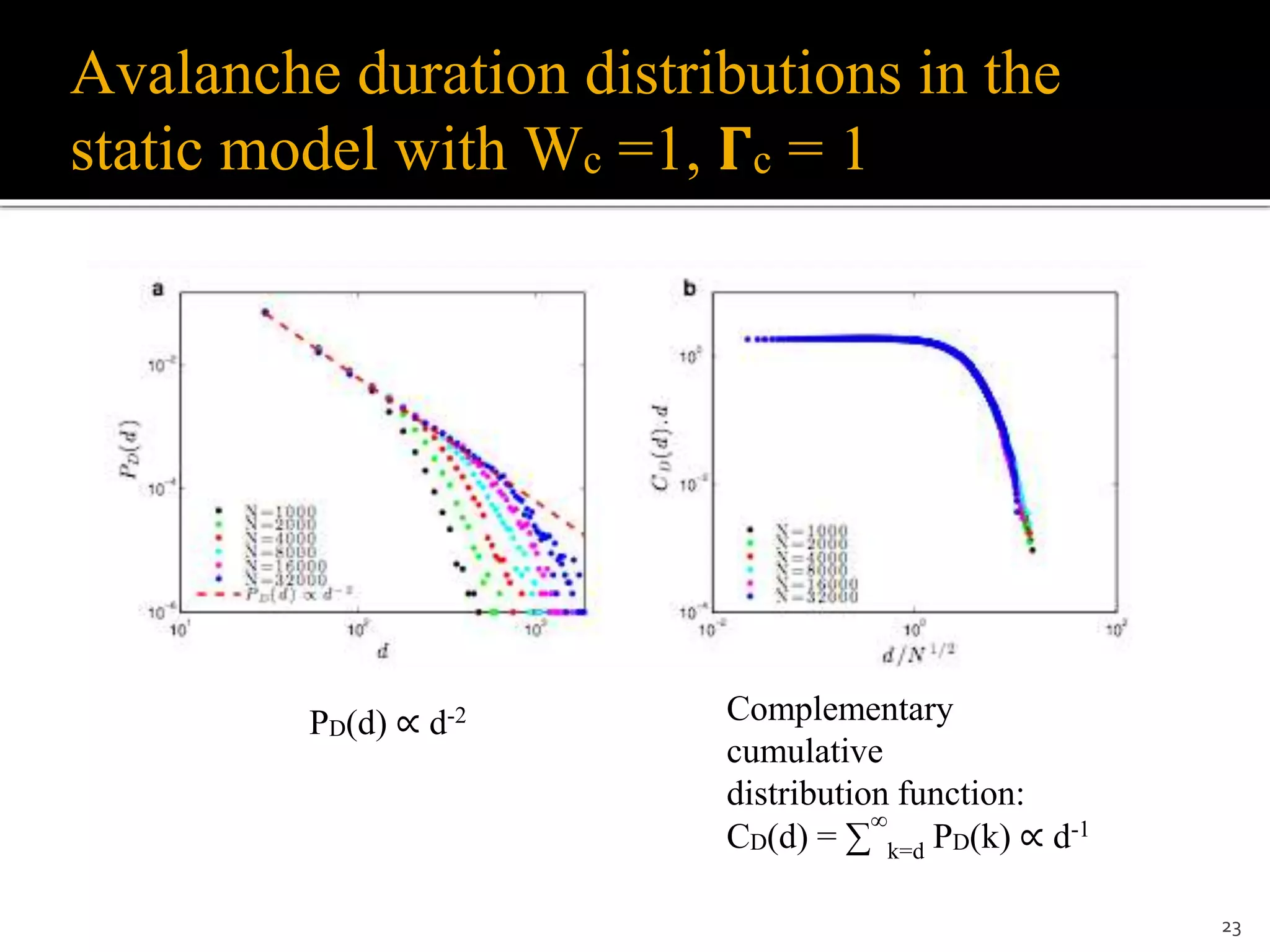
![Dynamic synapses and dynamic gains
Dynamic synapses (Levina et al., 2007; Levina et al.,
2009; Bonachela et al., 2010; Costa et al., 2015, Campos
et al., 2016):
Wij[t+1] = Wij[t] + 1/𝞽 (A − Wij[t]) − u Wij[t] Xj[t]
Dynamic gains (Brochini et al., 2016):
𝚪i[t+1] = 𝚪i[t] + 1/𝞽 (A − 𝚪i[t]) − u 𝚪i[t] Xi[t]
Parameters range:
0 < u < 1, A > Wc (or A > 𝚪c)
All works with dynamic synapses used
𝞽 = O(N)
26
Wc, 𝚪c
A, 𝞽 u
O(N2) equations
O(N) equations!](https://image.slidesharecdn.com/sosckinouchi2-171216155803/75/Neuronal-self-organized-criticality-25-2048.jpg)


![The same problem occurs with dynamic gains
𝚪i[t+1] = 𝚪i[t] + 1/𝞽 (A - 𝚪i[t]) - u 𝚪i[t] Xi[t]
Averaging + stationary state:
1/𝞽 (A - 𝚪*) = u 𝚪* ρ
With ρ = ( 𝚪*- 𝚪c )/𝚪*, we get:
𝚪* = (𝚪c - Ax)/(1+x), with x = 1/(u𝞽)
We have 𝚪* → 𝚪c only for x → 0, that is, if 𝞽 → ∞ (not biological)
29](https://image.slidesharecdn.com/sosckinouchi2-171216155803/75/Neuronal-self-organized-criticality-28-2048.jpg)


![Perpectives: a new neuronal network
formalism to be explored
More results, perhaps analytic, for the μ > 0 case.
Better study of dynamic synapses and dynamic gains
Other specific Φ functions (ex: Φ(V) = [𝚪(V-VT)]r/[1+[𝚪(V-VT)]r] = no 2-
cycles
Theorems for general Φ functions (ex: all linear piecewise functions give
analytic solutions)
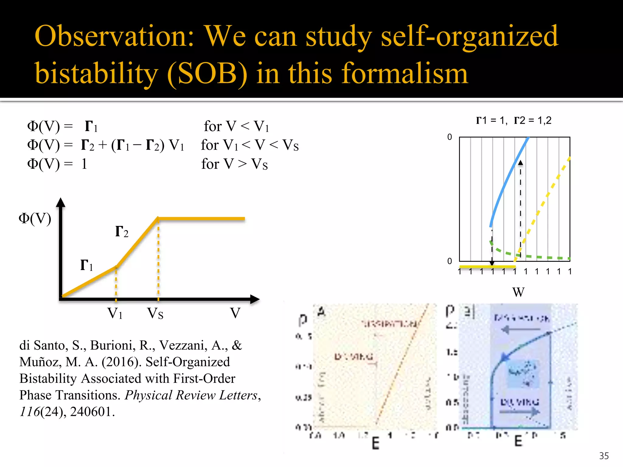
Self-organized bistability (SOB)
Other network topologies (scale free, small world etc.)
Other kinds of couplings
Inhibitory neurons (ex: Larremore et al., 2014)
Very large networks: N > 106, synapses > 1010
Realistic topologies (ex: cortical Potjans-Diesmann model with layers and
different neuron populations, N=8x10⁴, synapses = 3x10⁸, Cordeiro et al.,
2016)
Etc., etc., etc…
36](https://image.slidesharecdn.com/sosckinouchi2-171216155803/75/Neuronal-self-organized-criticality-34-2048.jpg)


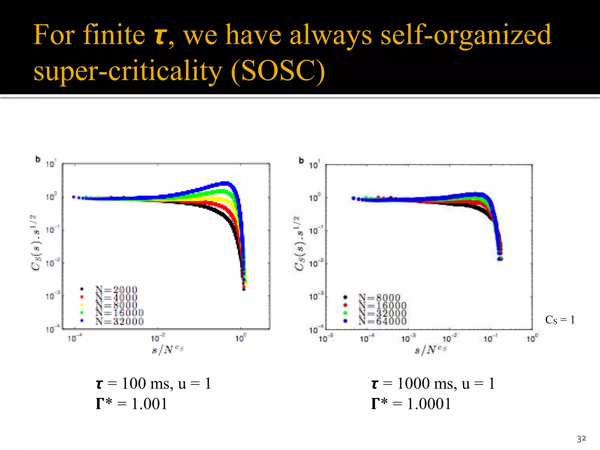
1) The document discusses a model of stochastic spiking neural networks where dynamical neuronal gains produce self-organized criticality. Introducing dynamic neuronal gains Γi[t] in addition to dynamic synaptic weights Wij[t] allows the system to self-organize toward a critical region without requiring divergent timescales. 2) For finite recovery timescales τ, the model exhibits self-organized supercriticality (SOSC) where the average neuronal gain Γ* is always slightly above critical. SOSC may help explain biological phenomena like large avalanches and epileptic activity. 3) The model provides a new framework to study self-organized phenomena in neuronal networks, including potential analytic solutions and