The document presents the Neural Processes family and discusses various types, including Conditional Neural Processes (CNPs) and Attentive Neural Processes (ANPs), emphasizing their ability to model uncertainty and improve predictive performance in tasks like function regression and image completion. Key concepts include the architecture of CNPs and their ability to integrate outputs and prior information for better learning efficiency compared to traditional Gaussian Processes. The document also details experimental results demonstrating the effectiveness of these models in few-shot learning scenarios and generative tasks.

1. Neural Processes Family
Kota Matsui
RIKEN AIP Data Driven Biomedical Science Team
August 20, 2019

2. Table of contents
1. Conditional Neural Processes [Garnelo+ (ICML2018)]
2. Neural Processes [Garnelo+ (ICML2018WS)]
3. Attentive Neural Processes [Kim+ (ICLR2019)]
4. Meta-Learning surrogate models for sequential decision
making [Galashov+ (ICLR2019WS)]
5. On the Connection between Neural Processes and Gaussian
Processes with Deep Kernels [Rudner+ (NeurIPS2018WS)]
6. Conclusion
K. Matsui (RIKEN AIP) Neural Processes Family 1 / 60

3. Table of Contents
1. Conditional Neural Processes [Garnelo+ (ICML2018)]
2. Neural Processes [Garnelo+ (ICML2018WS)]
3. Attentive Neural Processes [Kim+ (ICLR2019)]
4. Meta-Learning surrogate models for sequential decision
making [Galashov+ (ICLR2019WS)]
5. On the Connection between Neural Processes and Gaussian
Processes with Deep Kernels [Rudner+ (NeurIPS2018WS)]
6. Conclusion
K. Matsui (RIKEN AIP) Neural Processes Family Conditional Neural Processes 2 / 60

4. Motivation
Neural Net vs Gaussian Processes
£ Neural Net (NN)
• Function approximation ability
• New functions are learned from scratch each time
• Uncertainty of functions can not be considered
£ Gaussian Processes (GP)
• Can use prior knowledge to quickly estimate the shape of
new function
• Can model uncertainty of functions
• Computationally expensive
• Hard to design prior distribution
Aim
Combine the benefits of NN and GP
K. Matsui (RIKEN AIP) Neural Processes Family Conditional Neural Processes Introduction 3 / 60

5. Conditional Neural Processes (CNPs)
• A conditional distribution over functions trained to model
the empirical conditional distributions of functions
• permutation invariant in training/test data
• scalable: running time complexity of O(n + m)
K. Matsui (RIKEN AIP) Neural Processes Family Conditional Neural Processes Introduction 4 / 60

6. Stochastic Processes i
• observations : O = {(xi, yi)}n−1
i=0 ⊂ X × Y
• targets : T = {xi}n+m−1
i=n
• generative model (stochastic processes) :
• yi = f(xi), f : X → Y (noiseless case)
• f ∼ P (prior process)
• P Y P(f(T) | O, T) (predictive distribution)
Task
Predict the output values f(x) for ∀x ∈ T given O
Example 1 (Gaussian Processes)
P = GP(µ(x), k(x, x′))
Y predictive distribution : f(x) ∼ N(µn(x), σ2
n(x))
µn(x) = µ(x) + k(x)⊤
(K + σ2
I)−1
(y − m)
σ2
n(x) = k(x, x) − k(x)⊤
(K + σ2
I)−1
k(x)
K. Matsui (RIKEN AIP) Neural Processes Family Conditional Neural Processes Model 5 / 60

7. Stochastic Processes ii
1D Gaussian process regression
Difficulties of ordinary SP approaches
1. It is difficult to design appropriate priors
2. GPs (typical ex) do not scale w.r.t. the number of data
→ O((n + m)3) computational costs are required
K. Matsui (RIKEN AIP) Neural Processes Family Conditional Neural Processes Model 6 / 60

8. Conditional Neural Processes i
conditional stochastic process Qθ(f(·) | O, T)
Predictive Ability of NNs + Uncertainty Modeling of SPs
Assumption 1
1. (permutation invariant)
Qθ(f(T) | O, T) = Qθ
(
f
(
T′
)
| O, T′
)
= Qθ
(
f(T) | O′
, T
)
• O′
, T′
: permutations of O, T resp.
2. (factorizability)
Qθ(f(T) | O, T) =
∏
x∈T
Qθ(f(x) | O, x)
K. Matsui (RIKEN AIP) Neural Processes Family Conditional Neural Processes Model 7 / 60

9. Conditional Neural Processes ii Architecture
PredictObserve Aggregate
r3r2r1
…x3x2x1 x5 x6x4
ahhh y5 y6y4
ry3y2y1 g gg
…
ri = hθ(xi, yi) ∀(xi, yi) ∈ O
r = r1 ⊕ r2 ⊕ . . . rn−1 ⊕ rn
φi = gθ(xi, r) ∀(xi) ∈ T
hθ, gθ
⊕
r1 ⊕ r2 ⊕ . . . rn−1 ⊕ rn =
1
n
n
i=1
ri
Qθ (f (xi) | O, xi) = Q (f (xi) | φi)
φi = (µi, σ2
i ) N(µi, σ2
i )
K. Matsui (RIKEN AIP) Neural Processes Family Conditional Neural Processes Model 8 / 60

10. Conditional Neural Processes ii Architecture
• 構造としては VAE に非常に近い
→ h と a は VAE の encoder に対応し, 入力データから潜在
表現 r を獲得
• VAE との違いその 1 : 入力 x に加えて出力 y も与えて潜在
表現を学習
• VAE との違いその 2 : 潜在表現 r は確率変数ではなく, デー
タ毎の表現 r1, ..., rn の和で決まる
• 違いその 2 でデータ毎に独立に計算した潜在表現を使って
いることが後で説明する “画像全体で一貫した completion
にならない” 原因になっている
K. Matsui (RIKEN AIP) Neural Processes Family Conditional Neural Processes Model 9 / 60

11. Conditional Neural Processes iii Training
Optimization Problem
minimization of the negative conditional log probability
θ∗
= arg min
θ
L(θ)
L(θ) = −Ef∼P
[
EN
[
log Qθ
(
{yi}n−1
i=0 | ON , {xi}n−1
i=0
)]]
• f ∼ P : prior process
• N ∼ Unif(0, n − 1)
• ON = {(xi, yi)}N
i=0 ⊂ O
practical implementation : gradient descent
1. sampling f and N
2. MC estimates of the gradient of L(θ)
3. gradient descent by estimated gradient
K. Matsui (RIKEN AIP) Neural Processes Family Conditional Neural Processes Model 10 / 60

12. Function Regression i Setting
Dataset
1. random sample from GP w/ fixed kernel&params
2. random sample from GP w/ switching two kernels
network architectures
£ hθ : 3-layer MLP with 128-dim output ri, i = 1, ..., 128
£ r = 1
128
∑128
i=1 ri : aggregation
£ gθ : 5-layer MLP, gθ(xi, r) = µi, σ2
i (mean & var of Gaussian)
£ Adam (optimizer)
K. Matsui (RIKEN AIP) Neural Processes Family Conditional Neural Processes Experimental Results 11 / 60

13. Function Regression ii Results
K. Matsui (RIKEN AIP) Neural Processes Family Conditional Neural Processes Experimental Results 12 / 60

14. Image Completion i Setting
Dataset
1. MNIST (f : [0, 1]2 → [0, 1])
Complete the entire image from a small number of
observation
2. CelebA (f : [0, 1]2 → [0, 1]3)
Complete the entire image from a small number of
observation
network architectures
• the same model architecture as for 1D function regression
except for
• input layer : 2D pixel coordinates normalized to [0, 1]2
• output layer : color intensity of the corresponding pixel
K. Matsui (RIKEN AIP) Neural Processes Family Conditional Neural Processes Experimental Results 13 / 60

15. Image Completion ii Results
• 1 (non-informative) observation point
→ prediction corresponds to the average over all digits
K. Matsui (RIKEN AIP) Neural Processes Family Conditional Neural Processes Experimental Results 14 / 60

16. Image Completion ii Results
Random Context Ordered Context
# 10 100 1000 10 100 1000
kNN 0.215 0.052 0.007 0.370 0.273 0.007
GP 0.247 0.137 0.001 0.257 0.220 0.002
CNP 0.039 0.016 0.009 0.057 0.047 0.021 •
•
K. Matsui (RIKEN AIP) Neural Processes Family Conditional Neural Processes Experimental Results 15 / 60

17. Image Completion iii Latent Variable Model
Original CNPs
• The model returns factored outputs (sample-wise
independent modeling)
→ best prediction with limited data points is to average
over all possible predictions
• It can not sample different coherent images of all the
possible digits conditioned on the observations
← GPs can do this due to a kernel function
• Adding latent variables, CNPs can maintain this property
CNPs の latent variable model は後述する Neural Processes と
同じもの
K. Matsui (RIKEN AIP) Neural Processes Family Conditional Neural Processes Experimental Results 16 / 60

18. Image Completion iv Latent Variable Model
z ∼ N(µ, σ2
)
r = (µ, σ2
) = hθ(X, Y )
φi = (µi, σ2
i ) = gθ(xi, z)
•
K. Matsui (RIKEN AIP) Neural Processes Family Conditional Neural Processes Experimental Results 17 / 60

19. Classification i Settings
Dataset
• Omniglot
• 1,623 classes of characters from 50 different alphabets
• suitable for few-shot learning
• N-way classification task
• N classes are randomly chosen at each training step
network architectures
• encoder h : include convolution layers
• aggregation r : class-wise aggregation & concatenate
K. Matsui (RIKEN AIP) Neural Processes Family Conditional Neural Processes Experimental Results 18 / 60

20. Classification ii Results
PredictObserve Aggregate
r5r4r3
ahhh
r
Class
E
Class
D
Class
C g gg
r2r1
hh
Class
B
Class
A
A
B
C
E
D
0 1 0 1 0 1
5-way Acc 20-way Acc Runtime
1-shot 5-shot 1-shot 5-shot
MANN 82.8% 94.9% - - O(nm)
MN 98.1% 98.9% 93.8% 98.5% O(nm)
CNP 95.3% 98.5% 89.9% 96.8% O(n + m)
K. Matsui (RIKEN AIP) Neural Processes Family Conditional Neural Processes Experimental Results 19 / 60

21. Table of Contents
1. Conditional Neural Processes [Garnelo+ (ICML2018)]
2. Neural Processes [Garnelo+ (ICML2018WS)]
3. Attentive Neural Processes [Kim+ (ICLR2019)]
4. Meta-Learning surrogate models for sequential decision
making [Galashov+ (ICLR2019WS)]
5. On the Connection between Neural Processes and Gaussian
Processes with Deep Kernels [Rudner+ (NeurIPS2018WS)]
6. Conclusion
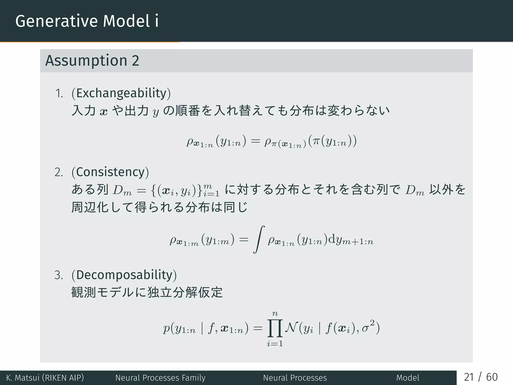
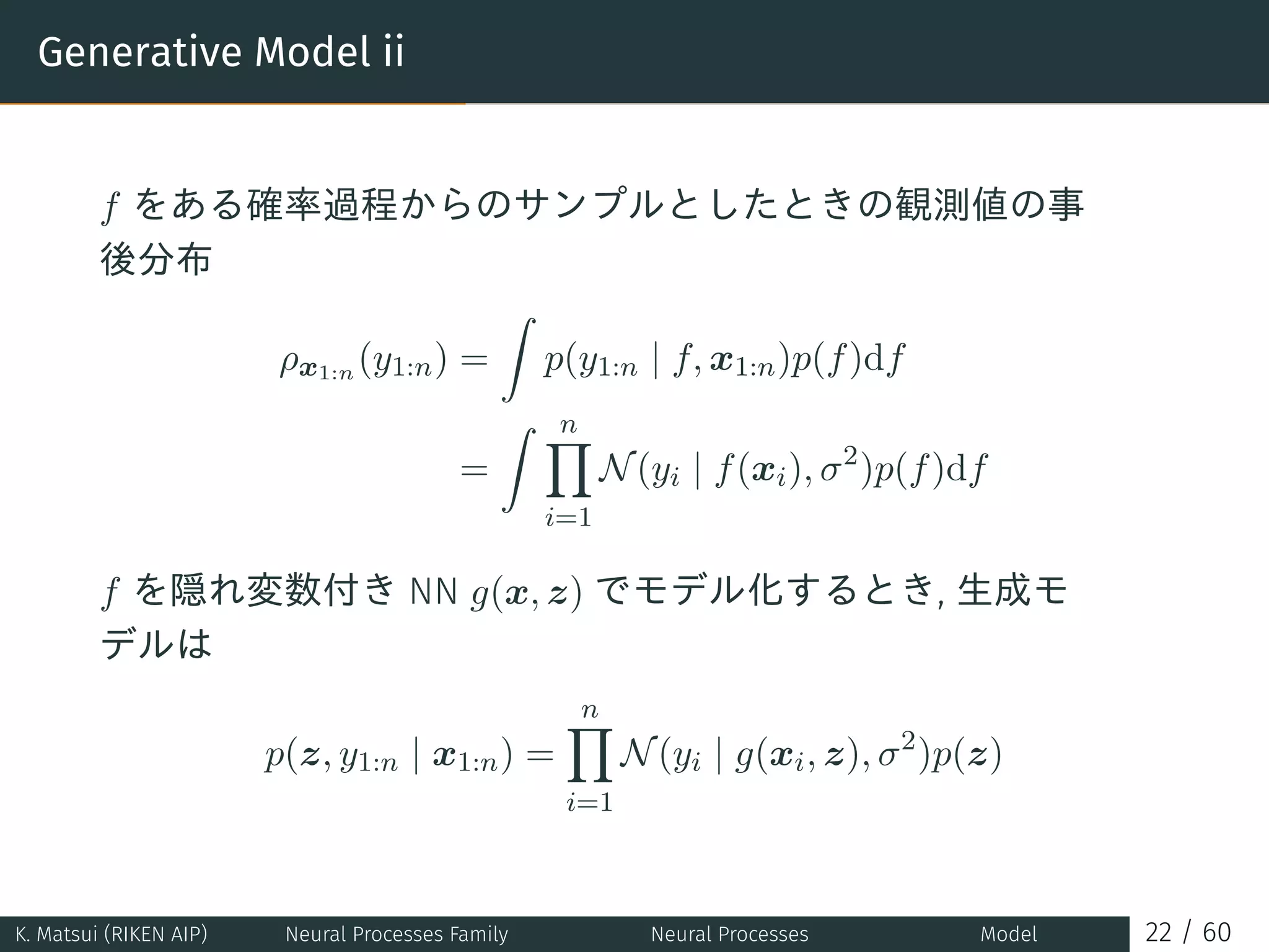
K. Matsui (RIKEN AIP) Neural Processes Family Neural Processes 20 / 60

22. Generative Model i
Assumption 2
1. (Exchangeability)
入力 x や出力 y の順番を入れ替えても分布は変わらない
ρx1:n (y1:n) = ρπ(x1:n)(π(y1:n))
2. (Consistency)
ある列 Dm = {(xi, yi)}m
i=1 に対する分布とそれを含む列で Dm 以外を
周辺化して得られる分布は同じ
ρx1:m (y1:m) =
∫
ρx1:n (y1:n)dym+1:n
3. (Decomposability)
観測モデルに独立分解仮定
p(y1:n | f, x1:n) =
n∏
i=1
N(yi | f(xi), σ2
)
K. Matsui (RIKEN AIP) Neural Processes Family Neural Processes Model 21 / 60

23. Generative Model ii
f をある確率過程からのサンプルとしたときの観測値の事
後分布
ρx1:n (y1:n) =
∫
p(y1:n | f, x1:n)p(f)df
=
∫ n∏
i=1
N(yi | f(xi), σ2
)p(f)df
f を隠れ変数付き NN g(x, z) でモデル化するとき, 生成モ
デルは
p(z, y1:n | x1:n) =
n∏
i=1
N(yi | g(xi, z), σ2
)p(z)
K. Matsui (RIKEN AIP) Neural Processes Family Neural Processes Model 22 / 60

24. Evidence Lower-Bound (ELBO)
隠れ変数 z の変分事後分布を q(z | x1:n, y1:n) とおくと ELBO は
log p (y1:n|x1:n)
≥ Eq(z|x1:n,y1:n)
[ n∑
i=1
log p (yi | z, xi) + log
p(z)
q (z | x1:n, y1:n)
]
特に予測時には観測データとテストデータを分割して
log p (ym+1:n | x1:m, xm+1:n, y1:m)
≥ Eq(z|xm+1:n,ym+1:n)
[ n∑
i=m+1
log p (yi | z, xi) + log
p (z | x1:m, y1:m)
q (z | xm+1:n, ym+1:n)
]
≈ Eq(z|xm+1:n,ym+1:n)
[ n∑
i=m+1
log p (yi | z, xi) + log
q (z | x1:m, y1:m)
q (z | xm+1:n, ym+1:n)
]
p を q で近似している理由は, 観測データによる条件付き分布としての計算
に O(m3
) のコストがかかるのを回避するため
K. Matsui (RIKEN AIP) Neural Processes Family Neural Processes Model 23 / 60

25. Architectures
x1 x2 x3
y1 y2 y3
hθ hθ hθ
r1 r2 r3
a
r
x4 x5 x6
gθ gθ gθ
z
ˆy4 ˆy5 ˆy6
z
z ∼ N(µ(r), σ2
(r)I)
gθ(xi) = P(y | z, xi) :
K. Matsui (RIKEN AIP) Neural Processes Family Neural Processes Model 24 / 60

26. Comparing Architectures : VAE, CNPs & NPs
X
qφ(z | X)
pθ(X | z)
ˆX
z ∼ N(0, I)
X Y
r =
n
i=1 ri
ˆY
gθ(Y | ˆX, r)
hθ(xi, yi)
X Y
r =
n
i=1 ri
ˆY
hθ(xi, yi)
z ∼ N(µ(r), σ2
(r)I)
gθ(Y | ˆX, z)
K. Matsui (RIKEN AIP) Neural Processes Family Neural Processes Model 25 / 60

27. Black-Box Optimization with Thompson Sampling
Neural process Gaussian process Random Search
0.26 0.14 1.00
K. Matsui (RIKEN AIP) Neural Processes Family Neural Processes Experiments 26 / 60

28. Table of Contents
1. Conditional Neural Processes [Garnelo+ (ICML2018)]
2. Neural Processes [Garnelo+ (ICML2018WS)]
3. Attentive Neural Processes [Kim+ (ICLR2019)]
4. Meta-Learning surrogate models for sequential decision
making [Galashov+ (ICLR2019WS)]
5. On the Connection between Neural Processes and Gaussian
Processes with Deep Kernels [Rudner+ (NeurIPS2018WS)]
6. Conclusion
K. Matsui (RIKEN AIP) Neural Processes Family Attentive Neural Processes 27 / 60

29. Recall : Neural Processes
x1 y1
x2 y2
x3 y3
MLPθ
MLPθ
MLPθ
MLPΨ
MLPΨ
MLPΨ
r1
r2
r3
s1
s2
s3
rCm
m sC
x
rC
~
MLP y
ENCODER DECODER
Deterministic
Path
Latent
Path
NEURAL PROCESS
m Mean
z
z
*
*
• 潜在表現 r と潜在変数 z を両方モデルに組み込む ver.
• ELBO を目的関数として学習
log p (yT | xT , xC , yC )
≥Eq(z|sT ) [log p (yT | xT , rC , z)] − DKL (q (z | sT ) ∥q (z | sC ))
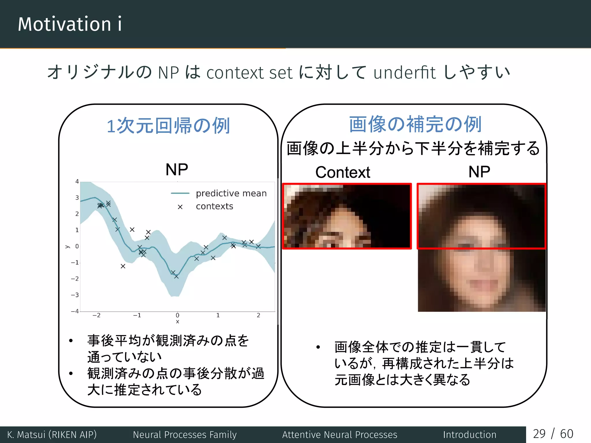
K. Matsui (RIKEN AIP) Neural Processes Family Attentive Neural Processes Introduction 28 / 60

30. Motivation i
オリジナルの NP は context set に対して underfit しやすい
•
•
•
K. Matsui (RIKEN AIP) Neural Processes Family Attentive Neural Processes Introduction 29 / 60

31. Motivation ii
underfit の原因に関する仮説
入力の潜在表現を平均してしまう操作がボトルネック
x1 x2 x3
y1 y2 y3
hθ hθ hθ
r1 r2 r3
a
r
⇒⇒
K. Matsui (RIKEN AIP) Neural Processes Family Attentive Neural Processes Introduction 30 / 60

32. Contribution
key observation : GP 回帰が underfit しないのはなぜ？
GP 回帰では, カーネル関数が 2 点の類似度を測る
→どの観測点 (xi, yi) が x∗ の予測に重要かを示す
• xi が x∗ に近ければ対応する予測値 y∗ も yi に近いことが
期待される
Contribution: Attentive neural processes (ANPs)
• (微分可能な) attention によって上記の性質を NP に実装
• 一方で, 観測点に対する permutation invariance は担保
• 1 次元の回帰と 2 次元の画像補完の問題で性能評価
K. Matsui (RIKEN AIP) Neural Processes Family Attentive Neural Processes Introduction 31 / 60

33. Attention
Notation
• key-value pair (xi, ri)
• key xi : 入力ベクトル
• value ri : 観測点 (xi, yi) の潜在表現 (encoder の出力)
• query x∗
attention mechanism
1. xi の x∗ に対する重み αi を計算
2. ri の重み付き和 r∗ =
∑n
i=1 αiri を x∗ の value とする
∗ r∗ は (xi, ri) の順序に依らない (permutation invariance)
K. Matsui (RIKEN AIP) Neural Processes Family Attentive Neural Processes Attention 32 / 60

34. Attention : Examples
£ Laplace
Wi = softmax({−∥Qi· − Xj·∥1}n
j=1) ∈ Rn
Laplace(Q, X, R) := W R ∈ Rm×dv
£ DotProduct
DotProduct(Q, X, R) := softmax
(
1
√
dk
QX⊤
R
)
∈ Rm×dv
£ MultiHead
MultiHead(Q, X, R) := concat(head1, ..., headH)W ∈ Rm×dv
headh = DotProduct(linear(Q), linear(X), linear(R))
• デザイン行列 X = (x1, ..., xn)⊤
∈ Rn×dk
• 対応する潜在表現行列 R = (r1, ..., rn)⊤
Rn×dv
• query 行列 Q = (x∗1, ..., x∗m)⊤
Rm×dk
K. Matsui (RIKEN AIP) Neural Processes Family Attentive Neural Processes Attention 33 / 60

35. Attentive Neural Processes : architectures
x1 y1
x2 y2
x3 y3
MLP
MLP
MLP
MLP
MLP
MLP
r1
r2
r3
s1
s2
s3
m sC
x
~
MLP y
ENCODER DECODER
Deterministic
Path
Latent
Path
Self-
attnϕ
Self-
attnω
Cross-
attention
x1 x2 x3 x
r
r
ATTENTIVE NEURAL PROCESS
m Mean
Keys Query
Values
z
z
*
*
*
*
*
K. Matsui (RIKEN AIP) Neural Processes Family Attentive Neural Processes Attention 34 / 60

36. Attentive Neural Processes : interpretation
£ self-attention による潜在表現の計算
• 観測点間の interaction のモデル化 (GP 回帰におけるカー
ネルによる観測点間の類似度計算に対応)
• もし多くの観測点が overlap している場合, 1 つまたは少数
の観測点に大きな重みを乗せるようにできる
£ cross-attention による query-specific な潜在表現の計算
• 各 query 点がその予測に重要と考えられる観測点により密
接に対応付けられるようにするパート
• global latent (そこから誘導される確率過程の大域的構造)
を担保するために, latent path には attention を入れない
K. Matsui (RIKEN AIP) Neural Processes Family Attentive Neural Processes ANPs 35 / 60

37. Attentive Neural Processes : Remarks
• self-attention, cross-attention を導入しても, 観測点に対す
る permutation invariant な性質は保たれる
• uniform attention (全ての観測点の同じ重みを割り振る) を
採用するとオリジナルの NP に帰着
• オリジナルの NP と同様の ELBO 最大化で学習
log p (yT | xT , xC, yC)
≥Eq(z|sT ) [log p (yT | xT , r∗, z)] − DKL (q (z | sT ) ∥q (z | sC))
• r∗ = r∗(xC, yC, xT ) : cross-attention の出力 (潜在表現)
• attention 計算 (各観測点に対する重み計算) が増えたため,
予測時の計算複雑さは O(n + m) から O(n(n + m)) に増加
K. Matsui (RIKEN AIP) Neural Processes Family Attentive Neural Processes ANPs 36 / 60

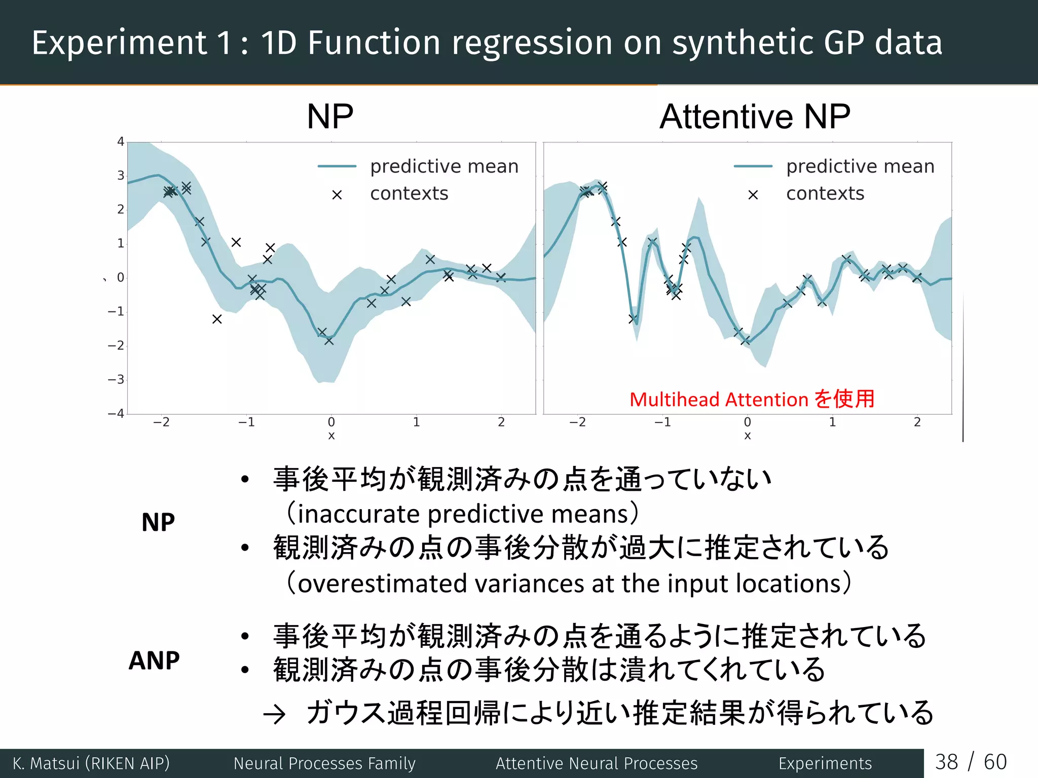
38. Experiment 1 : 1D Function regression on synthetic GP data
context point
target negative log likelihood
training iteration
wall clock time
Published as a conference paper at ICLR 2019
Figure 3: Qualitative and quantitative results of different attention mechanisms for 1D GP func
regression with random kernel hyperparameters. Left: moving average of context reconstruc
error (top) and target negative log likelihood (NLL) given contexts (bottom) plotted against train
iterations (left) and wall clock time (right). d denotes the bottleneck size i.e. hidden layer size o
MLPs and the dimensionality of r and z. Right: predictive mean and variance of different atten
mechanisms given the same context. Best viewed in colour.
1D Function regression on synthetic GP data We first explore the (A)NPs trained on data th
generated from a Gaussian Process with a squared-exponential kernel and small likelihood noi
We emphasise that (A)NPs need not be trained on GP data or data generated from a known stocha
process, and this is just an illustrative example. We explore two settings: one where the hype
rameters of the kernel are fixed throughout training, and another where they vary randomly at e
d =
hidden layer size of MLPs
dimensionality of r
dimensionality of z
• 2 GP
• context point n target point m iteration
•
• ANPs self-attention , cross-attention
1
|C|
i C
Eq(z|sC ) [log p (yi|xi, r (xC, yC, xi) , z)]
1
|T|
i T
Eq(z|sC ) [log p (yi|xi, r (xC, yC, xi) , z)]
K. Matsui (RIKEN AIP) Neural Processes Family Attentive Neural Processes Experiments 37 / 60

39. Experiment 1 : 1D Function regression on synthetic GP data
NP Attentive NP
Figure 1: Comparison of predictions given by a fully tr
tion regression (left) / 2D image regression (right). T
to predict the target outputs (y-values of all x 2 [ 2
are noticeably more accurate than for NP at the conte
provide relevant information for a given target predic
•
inaccurate predictive means
•
overestimated variances at the input locations
NP
ANP
•
•
→
Multihead Attention
K. Matsui (RIKEN AIP) Neural Processes Family Attentive Neural Processes Experiments 38 / 60

40. Experiment 1 : 1D Function regression on synthetic GP data
•
•
•
K. Matsui (RIKEN AIP) Neural Processes Family Attentive Neural Processes Experiments 39 / 60

41. Experiment 2 : 2D Function regression on image data
•
•
•
•
•
•
• p(yT | xT , rC, z)
•
•
K. Matsui (RIKEN AIP) Neural Processes Family Attentive Neural Processes Experiments 40 / 60

42. Experiment 2 : 2D Function regression on image data
K. Matsui (RIKEN AIP) Neural Processes Family Attentive Neural Processes Experiments 41 / 60

43. Table of Contents
1. Conditional Neural Processes [Garnelo+ (ICML2018)]
2. Neural Processes [Garnelo+ (ICML2018WS)]
3. Attentive Neural Processes [Kim+ (ICLR2019)]
4. Meta-Learning surrogate models for sequential decision
making [Galashov+ (ICLR2019WS)]
5. On the Connection between Neural Processes and Gaussian
Processes with Deep Kernels [Rudner+ (NeurIPS2018WS)]
6. Conclusion
K. Matsui (RIKEN AIP) Neural Processes Family BO via Neural Processes 42 / 60

44. Meta-Learning
個々のタスクに対して共通に良い初期値を与える上位の学習器
(meta-learner) を考える
Model-Agnostic Meta-Learning (MAML) [Finn+ (ICML2017)]
• meta-learner によって θ が task 1-3 の学習に対して良い初
期値となるように設定される
• meta-learner の設定した θ を warm start とすることでよ
り少ないコストで task 毎の最適なパラメータを発見
できる
K. Matsui (RIKEN AIP) Neural Processes Family BO via Neural Processes 43 / 60

45. BO from Meta-Learning Viewpoints
Key Observation
We can sample functions similar to the target function from
prior distribution (e.g. GP)
Algorithm 1 Bayesian Optimisation
Input:
f∗
- Target function of interest (= T ∗
).
D0 = {(x0, y0)} - Observed evaluations of f∗
.
N - Maximum number of function iterations.
Mθ - Model pre-trained on evaluations of similar
functions f1, . . . fn ∼ p(T ).
for n=1, ..., N do
// Model-adaptation
Optimise θ to improve M’s prediction on Dn−1.
Thompson sampling: Draw ˆgn ∼ M, find
xn = arg minx∈X E ˆg(y|x)
Evaluate target function and save result.
Dn ← Dn−1 ∪ {(xn, f∗
(xn))}
end for
K. Matsui (RIKEN AIP) Neural Processes Family BO via Neural Processes 44 / 60

46. NPs as Meta-Learning Model
Use neural processes as a model M because
1. statistical efficiency
Accurate predictions of function values based on small
numbers of evaluations
2. calibrated uncertainties
balance exploration and exploitation
3. O(n + m) computational complexity
4. non-parametric modeling
→ Not necessary to set hyper parameters such as learning
rate and update frequency in MAML
K. Matsui (RIKEN AIP) Neural Processes Family BO via Neural Processes 45 / 60

47. Experiments : Bayesian Optimization via NPs
Adversarial task search for RL agents [Ruderman+ (2018)]
• Search Problem of adversarially designed 3D Maze
• trivially solvable by human players
• But RL agents will catastrophically fail
• Notation
• fA : given agent mapping from task params to its
performance r
• parameters of the task
• M : maze layout
• ps, pg : start and goal positions
Problem setup
1. Position search (p∗
s, p∗
g) = arg min
ps,pg
fA(M, ps, pg)
2. Full maze search (M∗, p∗
s, p∗
g) = arg min
M,ps,pg
fA(M, ps, pg)
K. Matsui (RIKEN AIP) Neural Processes Family BO via Neural Processes 46 / 60

48. Experiments : Bayesian Optimization via NPs
(a) Position search results (b) Full maze search results
Figure 2: Bayesian Optimisation results. Left: Position search Right: Full maze search. We report
the minimum up to iteration t (scaled in [0,1]) as a function of the number of iterations. Bold
lines show the mean performance over 4 unseen agents on a set of held-out mazes. We also show
20% of the standard deviation. Baselines: GP: Gaussian Process (with a linear and Matern 3/2
product kernel [Bonilla et al., 2008]), BBB: Bayes by Backprop [Blundell et al., 2015], AlphaDiv:
AlphaDivergence [Hernández-Lobato et al., 2016], DKL: Deep Kernel Learning [Wilson et al., 2016].
K. Matsui (RIKEN AIP) Neural Processes Family BO via Neural Processes 47 / 60

49. Table of Contents
1. Conditional Neural Processes [Garnelo+ (ICML2018)]
2. Neural Processes [Garnelo+ (ICML2018WS)]
3. Attentive Neural Processes [Kim+ (ICLR2019)]
4. Meta-Learning surrogate models for sequential decision
making [Galashov+ (ICLR2019WS)]
5. On the Connection between Neural Processes and Gaussian
Processes with Deep Kernels [Rudner+ (NeurIPS2018WS)]
6. Conclusion
K. Matsui (RIKEN AIP) Neural Processes Family Connection between NP and GP 48 / 60

50. Contributions
Neural processes (NPs) と Gaussian processes (GPs) の理論的
な関係を示した. 特に, ある条件の下では NPs はカーネル関数
にdeep kernelsを用いた GPs と数学的に等価であることを示
した.
• GPs の理論が NPs に適用可能になりうる
• deep kernel GP を一度学習しておくことで異なる予測タス
クにも適用可能な共分散関数を獲得するという学習方法
方針
£ deep kernel GP と NP とで同じ ELBO が出てくる
£ 生成モデルとしては NP の decoder 部分を deep kernel の
NN と潜在変数の内積の形で書くと同じものになる
K. Matsui (RIKEN AIP) Neural Processes Family Connection between NP and GP 49 / 60

51. Gaussian Processes with Deep Kernels i
Notation
• x1:n, y1:n : 観測点
• f : Rp → R : 真関数
• GP model : p(f | x1:n) = N(m, K)
p(y1:n | f) = N(f, τ−1
I)
ここで, f = (f(x1), ..., f(xn)), m = (m(x1), ..., m(xn)),
Kij = k(xi, xj)
K. Matsui (RIKEN AIP) Neural Processes Family Connection between NP and GP GP with Deep Kernels 50 / 60

52. Gaussian Processes with Deep Kernels ii
Definition 1 (deep kernel [Tsuda+ (2002)])
k (xi, xj) :=
1
d
d∑
j,j′=1
σ
(
w⊤
j xi + bj
)
Σjj′ σ
(
w⊤
j′ xj + bj
)
• σ
(
w⊤
j xi + bj
)
は 1 層の NN, w, b はモデルパラメータで
σ(·) は活性化関数
• Σ = (Σjj′ )d
j,j′=1 は半正定値行列
行列表記
ϕi := ϕ(xi, W , b) =
√
1
d
σ(W ⊤
xi + b) ∈ Rd
,
Φ = [ϕ1, ..., ϕn] とおくと, k(X, X) = ΦΣΦ⊤.
以下, GP の平均関数は次のような形で書かれるとする
m(X) = Φµ, µ ∈ Rd
K. Matsui (RIKEN AIP) Neural Processes Family Connection between NP and GP GP with Deep Kernels 51 / 60

53. Gaussian Processes with Deep Kernels iii
Latent function を積分消去して得られるエビデンス (周辺尤度)
p (y|X) =
∫
p (y, f | X) df =
∫
p (y | f) p (f | X) df
= N
(
Φµ, ΦΣΦ⊤
+ τ−1
In
)
NPs の生成モデルと関連づけるために隠れ変数を導入
z ∼ N(µ, Σ)
このとき, 上記のエビデンスは z の周辺化からも導出される
p (y|X) =
∫
p (y | X, z) p (z) dz =
∫
N
(
Φz, τ−1
In
)
N (µ, Σ) dz
= N
(
Φµ, ΦΣΦ⊤
+ τ−1
In
)
特に, z ∼ N(0, Id) のときは p (y|X) = N(0, ΦΦ⊤ + τ−1In)
K. Matsui (RIKEN AIP) Neural Processes Family Connection between NP and GP GP with Deep Kernels 52 / 60

54. Gaussian Processes with Deep Kernels iv
エビデンス p (y|X) を計算するには共分散行列 ΦΣΦ⊤ + τ−1In
の逆行列計算が必要 (O(n3) の計算コスト)
→ エビデンス下界 (ELBO) の計算で置き換えてコスト削減
log p(Y | X) ≥ Eq(z|X)[log p(Y | z, X)] − KL(q(z | X)∥p(z))
K. Matsui (RIKEN AIP) Neural Processes Family Connection between NP and GP GP with Deep Kernels 53 / 60

55. 予測時の ELBO の一致 i
Deep kernel GPs のエビデンス下界を, 観測データとテストデー
タを明示的に分離して書く (C = 1 : m, T = m + 1 : n はそれぞ
れ観測データ, テストデータを表す)
log p (YT | XT , XC, YC)
≥Eq(z|XT ,YT ) [log p (YT | z, XT )] − KL (q (z | XT , YT ) ∥p (z | XC, YC))
ここで, p (z | XC, YC) は観測データ XC, YC に基づいて設定さ
れる “data-driven” な prior
p (z | XC, YC) = N(µ(XC, YC), Σ(XC, YC))
NPs でやったのと同様にこれを変分事後分布で近似する
p (z | XC, YC) ≈ q (z | XC, YC)
K. Matsui (RIKEN AIP) Neural Processes Family Connection between NP and GP NP as GP 54 / 60

56. 予測時の ELBO の一致 ii
以上の下で, Deep kernel GP の ELBO は
Eq(z|XT ,YT ) [log p (YT | z, XT )] − KL (q (z | XT , YT ) ∥q (z | XC, YC))
一方, NPs の ELBO は
log p (ym+1:n | x1:m, xm+1:n, y1:m)
≥ Eq(z|xm+1:n,ym+1:n)
[ n∑
i=m+1
log p (yi | z, xi) + log
p (z | x1:m, y1:m)
q (z | xm+1:n, ym+1:n)
]
≈ Eq(z|xm+1:n,ym+1:n)
[ n∑
i=m+1
log p (yi | z, xi) + log
q (z | x1:m, y1:m)
q (z | xm+1:n, ym+1:n)
]
となり, 両者の生成モデルが同じならばELBO も一致すること
がわかる
K. Matsui (RIKEN AIP) Neural Processes Family Connection between NP and GP NP as GP 55 / 60

57. 生成モデル
NPs の生成モデル:
p(Y | z, X)p(z) = N
(
Y ; gθ(z, X), τ−1
I
)
N(z; µ, Σ)
Deep kernel GPs with latent variable の生成モデル:
p(Y | z, X)p(z) = N
(
Y ; Φz, τ−1
I
)
N (z; µ, Σ)
上記を比較すると, gθ(z, X) = Φz ととれば両者が一致するこ
とがわかる. より一般には, パラメータ Θ = {W ℓ, bℓ}L
ℓ=1 を持つ
L 層の Deep NN ΦΘ(·) によって
gθ(z, X) = ΦΘ(X)z
なる形の affine-decoder を用いることで両者は一致する
K. Matsui (RIKEN AIP) Neural Processes Family Connection between NP and GP NP as GP 56 / 60

58. Table of Contents
1. Conditional Neural Processes [Garnelo+ (ICML2018)]
2. Neural Processes [Garnelo+ (ICML2018WS)]
3. Attentive Neural Processes [Kim+ (ICLR2019)]
4. Meta-Learning surrogate models for sequential decision
making [Galashov+ (ICLR2019WS)]
5. On the Connection between Neural Processes and Gaussian
Processes with Deep Kernels [Rudner+ (NeurIPS2018WS)]
6. Conclusion
K. Matsui (RIKEN AIP) Neural Processes Family Conclusion 57 / 60

59. Summary
• NPs family は出力 y を予測するための条件付き分布を直接
モデリングする方法
• GPs 回帰では予測時に O((m + n)3) かかっていた計算コス
トが O(m + n) で済む
• BO への応用も既に考えられている (問題によっては
GP-based の BO よりも高性能)
• 潜在表現 · 変数の導出に attention を用いた ANPs はより
GP に近い回帰の結果を返す
• NPs は GPs 回帰において deep kernel を用いるのと等価な
操作とみなせる
K. Matsui (RIKEN AIP) Neural Processes Family Conclusion 58 / 60

60. Further Neural Processes
• Functional neural processes [Louizos+ (arXiv2019)]
• Recurrent neural processes [Willi+ (arXiv2019)]
• Sequential neural processes [Singh+ (arXiv2019)]
• Conditional neural additive processes [Requeima+
(arXiv2019)]
K. Matsui (RIKEN AIP) Neural Processes Family Conclusion 59 / 60

61. References
[1] Chelsea Finn, Pieter Abbeel, and Sergey Levine. Model-agnostic meta-learning for fast adaptation of deep
networks. In Proceedings of the 34th International Conference on Machine Learning-Volume 70, pages
1126–1135. JMLR. org, 2017.
[2] Alexandre Galashov, Jonathan Schwarz, Hyunjik Kim, Marta Garnelo, David Saxton, Pushmeet Kohli, SM Eslami,
and Yee Whye Teh. Meta-learning surrogate models for sequential decision making. arXiv preprint
arXiv:1903.11907, 2019.
[3] Marta Garnelo, Dan Rosenbaum, Christopher Maddison, Tiago Ramalho, David Saxton, Murray Shanahan,
Yee Whye Teh, Danilo Rezende, and SM Ali Eslami. Conditional neural processes. In International Conference on
Machine Learning, pages 1690–1699, 2018.
[4] Marta Garnelo, Jonathan Schwarz, Dan Rosenbaum, Fabio Viola, Danilo J Rezende, SM Eslami, and Yee Whye
Teh. Neural processes. arXiv preprint arXiv:1807.01622, 2018.
[5] Hyunjik Kim, Andriy Mnih, Jonathan Schwarz, Marta Garnelo, Ali Eslami, Dan Rosenbaum, Oriol Vinyals, and
Yee Whye Teh. Attentive neural processes. arXiv preprint arXiv:1901.05761, 2019.
[6] Tim GJ Rudner, Vincent Fortuin, Yee Whye Teh, and Yarin Gal. On the connection between neural processes and
gaussian processes with deep kernels. In Workshop on Bayesian Deep Learning, NeurIPS, 2018.
K. Matsui (RIKEN AIP) Neural Processes Family Conclusion 60 / 60