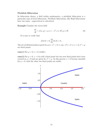
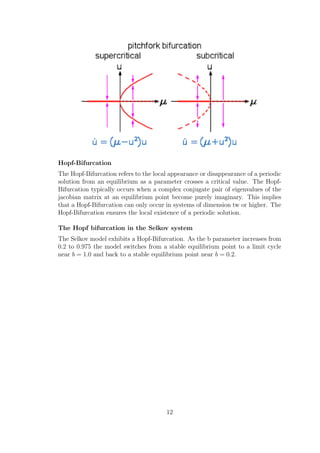
This document provides a summary of a project report on bifurcation analysis and its applications. It discusses key concepts in nonlinear systems such as equilibrium points, stability, linearization, and bifurcations including saddle node, transcritical, pitchfork and Hopf bifurcations. Examples are given to illustrate each type of bifurcation. Population models involving competition and prey-predator interactions are also discussed. The document outlines the contents which cover preliminary remarks, local theory of nonlinear systems, different types of bifurcations, and applications to population models.

1. VISVESVARAYA NATIONAL INSTITUTE OF
TECHNOLOGY
Project Report
Bifurcation analysis and applications
May 5,2016
Project Supervisor:
Dr.G.Naga Raju
Department of Mathematics
Prashant Patel
MS14MTH013
M.Sc. Mathematics

2. CONTENTS
1 Preliminary Remarks
2 Nonlinear Systems: Local Theory
2.1 Some Preliminary Concpts and Definitions
2.2 Stability, Liapunov Stability, Asymptotically Stable
2.3 Linearization
2.4 Hartman-Grobman Theorem
2.5 Routh-Hurwitz Criterian
3 Bifurcation of equilibrium points
3.1 Saddle Node Bifurcation
3.2 Transcritical Bifurcatiion
3.3 Pitchfork Bifurcation
3.4 Hopf Bifurcation
3.5 Selkov Model of Hopf Bifurcation
3.6 Sotomayor Theorems
3.7 Hopf Bifurcation Theorem
4 Population models
4.1 Two-species Competition Models
4.2 Prey-Predator Models
5 Conclusion
6 References
1

3. Preliminary Remarks
Differential equations are used in physics, chemistry,
biology, economics, engineering to model the real world problems. Few of the
applications of differential equations are as follows:
1 Population models
2 Prediction of weather
3 Prediction of stock prices
4 Atmospheric pollution
5 Diffusion of materials
6 Epidemic models
7 Pattern formation (e.g. stripes in Zebra, spots in leopards)
8 In general nonlinear systems cannot be solved explicitly therefore qualitative
behaviour of the system can change as parameters are varied.
9 The dynamics of the one dimensional ODE is very limited: all solutions either
settle down to equilibrium or head out to ±∞
10 In higher dimensional phase space a wider range of dynamical behaviour is
possible.
11 What is interesting about nonlinear systems?
Answer: dependence on parameters.
12 modeling in ecology is to predict the behaviour of system for different
parametric conditions.
2

4. Non Linear Systems:Local theory
Equillibrium Solution
Consider a general autonomous vector field
dx
dt
= f(x, ν), x ∈ Rn
, ν ∈ R, (1)
an equillibrium solution is a point x ∈ Rn
such that f(x) = 0, that is a solution
which does not change in time.
Stability
let x(t) be any solution of dx/dt = f(x) then x(t) is stable if solutions starting
close to x(t) at a given time remain close to x(t) for all later time.
It is asymptotically stable if nearby solutions actually converge to x(t) as t tends
to ∞.
Liapunov Stability
x(t) is said to be stable if given ε > 0 there exist a δ > 0 such that for any other
solution y(t) of dx/dt = F(x) satisfying, then for t > t0, t0 ∈ R
|x(t) − y(t)| < ε,
|x(t0) − y(t0)| < δ.
Asymptotic Stability
x(t) is said to be asymptotically stable if it is Liapunov stable and if there exist a
constant b > 0 such that if
|x(t0) − y(t0)| < b,
then limt→∞|x(t) − y(t)| = 0.
Theorem 1. (For Asymptotically Stable) Suppose all of the eigen-values of
f (x) have negative real parts. Then the equillibrium solution x = x of the non
linear vector field
dx/dt = f(x), x ∈ Rn
is asymptotically stable.
Hyperbolic Fixed Points
Let x = x be a fixed point of dx/dt = f(x), x ∈ Rn
. Then x is called a hyperbolic
fixed point if none of the eigen values of f (x) = J have zero real part.
Saddle, Stable and unstable node and Center
A hyperbolic fixed point of a vector field is called saddle if some, but not all of the
eigenvalues of the associated linearization have real parts greater than zero. If all
the eigenvalues have negative real parts then the hyperbolic fixed point are called
stable node. and if all the eigenvalues have positive real parts then the hyperbolic
fixed points are called unstable node. If the eigenvalues are purely imaginary and
non zero the non hyperbolic fixed point is called a center.
3

5. Stable and unstable node
4

6. Examples of Saddlele, stable node, stable spiral and center
5

7. Linearization
Let dx
dt
= f(x) be a vector field. Let x∗
be a fixed point and let η(t) = x(t) − x∗
be a small perturbation away from x∗
. To see whether the perturbation grows or
decays we derive a differential equation for η.
η(t) = x(t) − x∗
(2)
dη
dt
=
d(x − x∗
)
dt
=
dx
dt
,
since x∗
is constant,
Thus
dη
dt
=
dx
dt
= f(x) = f(x∗
+ η),
Now using Taylor’s expansion we obtain
dη
dt
= f(x∗
+ η) = f(x∗
) + η ∗ f (x∗
) + O(η2
), (3)
where o(η2
) denotes quadratically small terms in η. Finally note that f(x∗
) = 0
since x∗
is a fixed point. Hence
dη
dt
= η ∗ f (x∗
) + O(η2
),
Now if f (x∗
) = 0 the O(η2
) terms are negligible and we write the approximation
dη
dt
= η ∗ f (x∗
). (4)
This is a linear equation in η and is called the linearization about x∗
. It shows
that the perturbation grows exponentially if f (x∗
) > 0 and decays if f (x∗
) < 0.
If f (x∗
) = 0 the O(η2
) terms are not negligble and a non linear analysis is needed
to determine stability.
Example Using linear stability analysis determine the stability of the fixed points
for f(x) = sin(x).
The fixed points occur where f(x) = sin(x) = 0. Thus x∗
= kΠ is the fixed point,
where k is an integer.
f (x∗
) = cos(kΠ) = {1, k is even, −1, k is odd},
Hence x∗
is unstable if k is even and stable if k is odd.
Here in figure (a) −2Π, 2Π, 4Π are unstable fixed points and −Π, Π, 3Π are stable
fixed points.
6

8. Routh-Hurwitz Stability Criterion
If A is an m × m matrix, then the characteristic equation of A is given by:
λm
+ a1λm−1
+ a2λm−2
+ ....... + am = 0, where, ais, i = 1, 2, · · · · ·m are real
numbers.
Define
D1 = a1,
D2 = det
a1 a3
1 a2
and
Dk = det










a1 a3 a5 . . . a2k−1
1 a2 a4 . . . a2k−2
0 a1 a3 . . . a2k−3
0 1 a2 . . . a2k−4
. . . . . . .
. . . . . . .
0 0 0 . . . ak










, k = 1, 2, · · · · ·m.
where,aj = 0 for j > m. Then, the roots of characteristic equation have negative
real parts if and only if Dk > 0 for all k = 1, 2, · · · · m.
7

9. Theorem 2. Hartman Grobman theorem
Consider a vector field
dx
dt
= f(x), x ∈ Rn
, (5)
Where f is defined on a sufficiently large open set of rn
. Suppose that equation
(5) has a hyperbolic fixed point at x = x0 i.e.
f(x0) = 0,
and when f (x0) has no eigen values on the imaginary axis. Consider the associ-
ated linear vector field
dξ
dt
= f(x0) ∗ ξ, ξ ∈ Rn
. (6)
Then we have following theorem:
The flow generated by equation (5) is c0
conjugate to the flow generated by equation
(6) in a neighbourhood of the fixed point x = x0 or to say that the two autonomous
system of differential equations such as (5) and (6) are said to be topologically
equivalent in a neighbourhood of the origin or to have the same qualitative struc-
ture near the origin.
Bifurcation of Equilibrium Points
The change in qualitative behaviour (e.g. equilibrium points or periodic solutions
or their stability properties) as a parameter passes through a critical point is
known as bifurcation.
Saddle-Node Bifurcation
It is Basic mechanism by which equilibrium points are created or destroyed . As
the bifurcation parameter passes through the bifurcation point, two equilibria
disappear, so there are no equilibria afterward. One of the two equilibria is stable
another is unstable, before they disappear.
Example Consider the vector field
dy
dt
= f(y, a) = a − y2
, y ∈ R , a ∈ R , (7)
8

10. It is easy to verify that
f(0, 0) = 0,
∂f
∂y
(0, 0) = 0 ,
The set of all fixed points is given by a − y2
= 0 ⇒ a = y2
. This represents a
parabola in the a − y plane.
For
y =
√
a ⇒ f = −2
√
a (stable),
For
y = −
√
a ⇒ f = 2
√
a (unstable).
In the figure arrows along the vertical lines represents the flow generated by (7)
along the x- direction. Thus for a < 0 (7) has no fixed points and the vector field
is decreasing in x. For a > 0 (7) has two fixed points. A simple linear stability
analysis shows that one of the fixed points is stable and the other fixed point is
unstable. THis is an example of Saddle-Node Bifurcation. (x, a) = (0, 0) is a
bifurcation point and a = 0 is bifurcation value.
9

11. Transcritical Bifurcation
In a Transcritical Bifurcation, there are two equilibria one stable and other unsta-
ble. When the Bifurcation point is passed, the unstable becomes stable and stable
one becomes unstable.
Example consider the vector field
dy
dt
= f(y, a) = ay − y2
, y ∈ R , a ∈ R , (8)
It is easy to verify that
f(0, 0) = 0,
∂f
∂y
(0, 0) = 0,
The set of all fixed points is given by ay − y2
= 0 ⇒ y(a − y) = 0 ⇒ y = 0, a = 0
are fixed points.
case(1) For a < 0, y = 0 (stable), y = a (unstable)
case(2) For a > 0, y = 0 (unstable), y = a (stable)
Thus an exchange of stability has occured at a = 0.
10

12. Pitchfork Bifurcation
In bifurcation theory, a field within mathematics, a pitchfork bifurcation is a
particular type of local bifurcation. Pitchfork bifurcations, like Hopf bifurcations
have two types - supercritical or subcritical.
Example Consider the vector field
dx
dt
= f(x, µ) = µ ∗ x − x3
, x ∈ R , µ ∈ R , (9)
It is easy to verify that
f(0, 0) = 0,
∂f
∂x
(0, 0) = 0 ,
The set of all fixed points is given by µ∗x−x3
= 0 ⇒ x(µ−x2
) = 0 ⇒ x = 0, x2
= µ
are fixed points.
case(1) For µ < 0, x = 0 (stable)
case(2) For µ > 0, x = 0 is still a fixed point but two new fixed points have been
created at µ = 0 and are given by x2
= µ. In this process x = 0 become unstable
for µ > 0, with the other two fixed points are stable.
11

13. Hopf-Bifurcation
The Hopf-Bifurcation refers to the local appearance or disappearance of a periodic
solution from an equilibrium as a parameter crosses a critical value. The Hopf-
Bifurcation typically occurs when a complex conjugate pair of eigenvalues of the
jacobian matrix at an equilibrium point become purely imaginary. This implies
that a Hopf-Bifurcation can only occur in systems of dimension tw or higher. The
Hopf-Bifurcation ensures the local existence of a periodic solution.
The Hopf bifurcation in the Selkov system
The Selkov model exhibits a Hopf-Bifurcation. As the b parameter increases from
0.2 to 0.975 the model switches from a stable equilibrium point to a limit cycle
near b = 1.0 and back to a stable equilibrium point near b = 0.2.
12

14. Theorem 3. (Sotomayor Theorems):
Let us consider a system
dx
dt
= f(x, ν), x ∈ Rn
, ν ∈ R, (10)
Suppose the f(x∗, ν∗) =0 and that the n × n matrix A ≡ Df(x∗, ν∗) has a
simple eigenvalue λ = 0 with eigenvector v and that AT
has an eigenvector w
corresponding to the eigenvalue λ = 0. Furthermore, suppose that A has k
eigenvalue with negative real part and (n-k-1) eigenvalues with positive real parts
and that the following conditions are satisfied
wT
fν(x∗, ν∗) = 0 and wT
[D2
f(x∗, ν∗)(v, v)] = 0, (11)
Then the system (10) experiences a Saddle-node bifurcation at the equilibrium
point x∗ as the parameter ν passes through the bifurcation value ν = ν∗
13

15. If the conditions (11) are changed to
wT
fν(x∗, ν∗) = 0andwT
[Dfν(x∗, ν∗)v] = 0, wT
[D2
f(x∗, ν∗)(v, v)] = 0. (12)
Then above system (10) experiences a transcritical bifurcation at the equilibrium
point x∗ as the parameterν varies through the bifurcation value ν = ν∗
Theorem 4. (Hopf-Bifurcation Theorem(1942))
Suppose(10) has an equilibrium at (x∗, ν∗) satisfying following:
(H1) : Dxf(x∗, ν∗) ,
has a simple pair of purely imaginary eigenvalues and no other eigenvalues with
zero real parts.
Then (H1) implies that there is a smooth curve of equilibrium points (x(ν), ν)
with x(ν∗)=x. The eigenvalues λ(ν), λ(ν) of Dxf(x(ν)ν∗) which are imaginary at
ν = ν∗ vary smoothly with ν. If, moreover,
(H2) :
d
dν
(Reλ(ν))|ν=ν∗ = 0 .
is satisfied,then there exists a unique branch of periodic solution of the system(10)
near (x∗, ν∗).
14

16. Population Models
Two-Species Competition Models
A general model for two interacting species that compete for a common food
supply with population sizes x1(t) and x2(t) is given by
dx1
dt
= x1F(x1, x2),
dx2
dt
= x2G(x1, x2), (13)
Subject to the positive initial condition
x1(0) > 0, x2(0) > 0 ,
Where F(x1, x2) and G(x1, x2) are the growth rates of both the species respec-
tively. The growth rates F(x1, x2) and G(x1, x2) satisfy the following assumptions:
(1) An increase in population of one species will result in a decrease of the growth
rate of the other as the two species compete for the same resources. Hence
∂F
∂x2
(x1, x2) < 0,
∂G
∂x1
(x1, x2) < 0 ,
(2) If either of the population becomes very large, both population tend to de-
crease. Hence there exist k > 0 such that
F(x1, x2) < 0, G(x1, x2) < 0,
if x1 ≥ k or x2 ≥ k
(3) In the absence of the other species, both species have a positive growth rate
up to a certain population and then a negative growth rate beyond it. Therefore
there are constants k1 > 0, k2 > 0 such that
F(x1, 0) > 0 for x1 < k1 andF(x1, 0) < 0 for x1 > k1 ,
G(0, x2) > 0 for x2 < k2 andG(0, x2) < 0 for x2 > k2 .
Examples of Competition Model
The most popular example for two competing species is the classical Lotka-Volterra
competition model.The Lotka-Volterra equations, also known as the predator -prey
equations, are a pair of first-order, non-linear, differential equations frequently
used to describe the dynamics of biological systems in which two species interact,
one as a predator and the other as prey. The populations change through time
according to the pair of equations:
15

17. dx
dt
= αx − βxy ,
dy
dt
= δxy − γy .
Where, x is the number of prey, y is the number of some predator. dy
dt
and dx
dt
represent the growth rates of the two populations over time, t represents time and
α, β, γ, δ are positive real parameters describing the interaction of the two species.
Physical meaning of the equations
The Lotka-Volterra model makes a number of assumptions about the environment
and evolution of the predator and prey populations:
(1) The prey population finds ample food at all times.
(2) The food supply of the predator population depends entirely on the size of the
prey population.
(3) The rate of change of population is proportional to its size.
(4) During the process, the environment does not change in favour of one species
and genetic adaptation is inconsequential.
(5) Predators have limitless appetite.
As differential equations are used, the solution is deterministic and continuous.
This, in turn, implies that the generations of both the predator and prey are con-
tinually overlapping.
Prey
When multiplied out, the prey equation becomes
dx
dt
= αx − βxy ,
The prey are assumed to have an unlimited food supply, and to reproduce expo-
nentially unless subject to predation; this exponential growth is represented in the
equation above by the term αx. The rate of predation upon the prey is assumed
to be proportional to the rate at which the predators and the prey meet; this is
represented above by βxy. If either x or y is zero then there can be no predation.
With these two terms the equation above can be interpreted as: the change in the
prey’s numbers is given by its own growth minus the rate at which it is preyed
upon.
Predators
The predator equation becomes
dy
dt
= δxy − γy ,
In this equation,δxy represents the growth of the predator population. (Note the
similarity to the predation rate; however, a different constant is used as the rate at
16

18. which the predator population grows is not necessarily equal to the rate at which
it consumes the prey).γy represents the loss rate of the predators due to either
natural death or emigration; it leads to an exponential decay in the absence of
prey.
Hence the equation expresses the change in the predator population as growth
fueled by the food supply, minus natural death.
Solutions to the equations
The equations have periodic solutions and do not have a simple expression in
terms of the usual trigonometric functions, although they are quite tractable.If
none of the non-negative parameters α, β, γ, δ vanishes, three can be absorbed
into the normalization of variables to leave but merely one behind: Since the first
equation is homogeneous in x, and the second one in y, the parameters β
α
and
δ
γ
, are absorbable in the normalizations of y and x, respectively, and γ into the
normalization of t, so that only α
γ
remains arbitrary. It is the only parameter
affecting the nature of the solutions.
A linearization of the equations yields a solution similar to simple harmonic mo-
tion with the population of predators trailing that of prey by 900
in the cycle.
Frequency Plot
A simple example
Suppose there are two species of animals, a baboon (prey) and a cheetah (preda-
tor). If the initial conditions are 80 baboons and 40 cheetahs, one can plot the
progression of the two species over time. The choice of time interval is arbitrary.
17

19. Frequency Plot
One may also plot solutions parametrically as orbits in ”phase-space”, without
representing time, but with one axis representing the number of prey and the
other axis representing the number of predators for all times. This is to say, elim-
inating time from the two differential equations above results in only one such,
dy
dx
=
−y(δx − y)
x(βy − α)
,
whose solutions are closed curves; integrating d∗log(y)(α−βy)−d∗log(x)(γ−αx)
yields an evident constant quantity V depending on the initial conditions, which
is conserved on each curve,
V = −δx + γlog(x) − βy + αlog(y) .
18

20. Phase Space Plot
An aside: These graphs illustrate a serious potential problem with this as a bi-
ological model: For this specific choice of parameters, in each cycle, the baboon
population is reduced to extremely low numbers, yet recovers (while the cheetah
population remains sizeable at the lowest baboon density). In real-life situations,
however, chance fluctuations of the discrete numbers of individuals, as well as the
family structure and life-cycle of baboons, might cause the baboons to actually go
extinct, and, by consequence, the cheetahs as well. This modelling problem has
been called the ”atto-fox problem an atto-fox being a notional 10−
18 of a fox, in
the context of rabies modelling in the UK.
Phase-space plot of a further example
A less extreme example covers:α = 2/3, β = 4/3, γ = 1 = δ. Assume x,y quantify
thousands, each. Circles represent prey and predator initial conditions from x =
y =0.9 to 1.8, in steps of 0.1. The fixed point is at (1,1/2).
19

21. Phase-space plot
Dynamics of the system
In the model system, the predators thrive when there are plentiful prey but, ulti-
mately, outstrip their food supply and decline. As the predator population is low
the prey population will increase again. These dynamics continue in a cycle of
growth and decline.
Population equilibrium
Population equilibrium occurs in the model when neither of the population levels
is changing, i.e. when both of the derivatives are equal to 0.
x(α − βy) = 0, −y(γ − δx) = 0 ,
When solved for x and y the above system of equations yields y=0, x=0 and
y =
α
β
, x =
γ
δ
.
20

22. Hence, there are two equilibria,
The first solution effectively represents the extinction of both species. If both
populations are at 0, then they will continue to be so indefinitely. The second
solution represents a fixed point at which both populations sustain their current,
non-zero numbers, and, in the simplified model, do so indefinitely. The levels of
population at which this equilibrium is achieved depend on the chosen values of
the parameters,α, β, γ, δ.
Stability of the fixed points
The stability of the fixed point at the origin can be determined by performing a
linearization using partial derivatives, while the other fixed point requires a slightly
more sophisticated method. The Jacobian matrix of the predator-prey model is
J(x, y) =
α − βy −βx
δy δx − γ
.
First fixed point (extinction)
When evaluated at the steady state of (0, 0) the Jacobian matrix J becomes:
J(0, 0) =
α 0
0 −γ
.
The eigenvalues of this matrix are λ1 = α, λ2 = −γ. In the model α and γ are
always greater than zero, and as such the sign of the eigenvalues above will always
differ. Hence the fixed point at the origin is a saddle point.
The stability of this fixed point is of significance. If it were stable, non-zero pop-
ulations might be attracted towards it, and as such the dynamics of the system
might lead towards the extinction of both species for many cases of initial popula-
tion levels. However, as the fixed point at the origin is a saddle point, and hence
unstable, it follows that the extinction of both species is difficult in the model.
(In fact, this could only occur if the prey were artificially completely eradicated,
causing the predators to die of starvation. If the predators were eradicated, the
prey population would grow without bound in this simple model): The popula-
tions of prey and predator can get infinitesimally close to zero and still recover.
Second fixed point (oscillations)
Evaluating J at the second fixed point leads to:
J(
γ
δ
,
α
β
) =
0 −βγ
δ
α
δ
β 0
,
The eigenvalues of this matrix are
λ1 = i
√
αγ, λ2 = −i
√
αγ .
21

23. As the eigenvalues are both purely imaginary, this fixed point is not hyperbolic,
so no conclusions can be drawn from the linear analysis. However, as illustrated
above, the system admits a constant of motion V, or, equivalently, exp(V),
K = yα
exp(−βy)xγ
exp(−δx) ,
and the level curves, for each constant K, are closed orbits surrounding the fixed
point: the levels of the predator and prey populations cycle, and oscillate around
this fixed point. Increasing K moves a closed orbit closer to the fixed point. The
largest value of the constant K is obtained by solving the optimization problem.
K = yα
exp(−βy)xγ
exp(−δx) =
yα
xγ
exp(δx + βy)
−→ max (x, y) > 0 ,
.
The maximal value of K is thus attained at the stationary (fixed) point (γ
δ
, α
β
) and
amounts to
K∗
= (
α
βe
)α
(
γ
δe
)γ
.
where e is Euler’s Number.
22

24. Methodology
1 To analyze the various aspects of models we use the tools of nonlinear ODE.
2 The stability of various equilibrium points have been discussed with the help
of linearization techniques, Hartman-Grobman theorem, Routh-Hurwitz criterion
and Bendixson-Dulac criterion.
3 Sotomayor’s theorem has been used to prove the existence of saddle node and
transcritical bifurcation.
4 The existence of periodic solution through Hopf- bifurcation has been proved by
using Hopf-bifurcation theorem.
5 Normal form theory is used to reduce the models into their corresponding canon-
ical form of Bogdanov-Takens bifurcation.
6 Numerical simulations in MATLAB and MAPLE have been carried out to verify
the results obtained analytically.
23

25. References:
1 L. Perko, Differential equation and dyanamical system, Springer(1996).
2 J. Guckenheimer and P. Holmes , Nonlinear Oscillations dynamical system
and Bifurcatioins of vector fields ( Springer, New York 1983).
3 Steven H.strogatz, Nonlinear dynamics and chaos, with applications to Physics,
Chemistry, Biology and engineering
4 Stephen Wiggins, Introduction to Applied Nonlinear Dynamical Systems and
Chaos
24