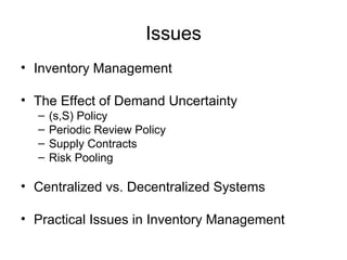
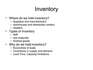
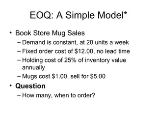
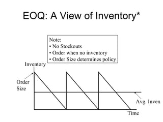
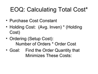
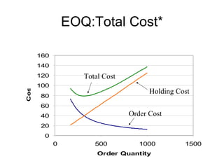
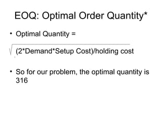
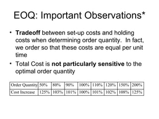
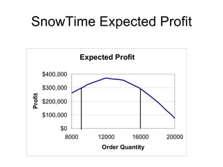
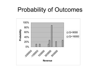
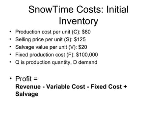
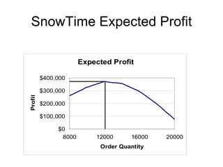
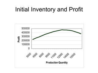
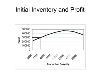
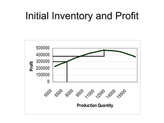
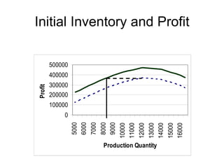
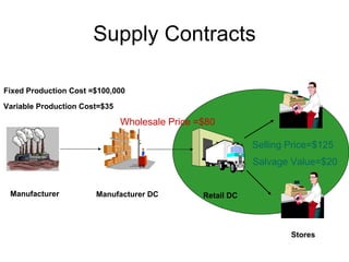
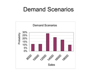
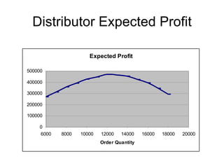
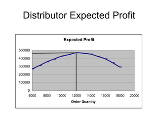
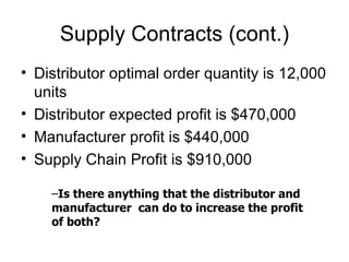
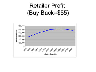
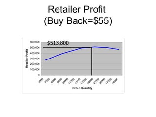
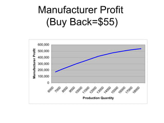
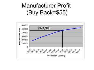
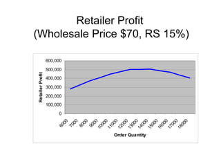
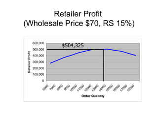
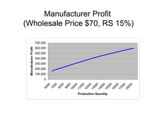
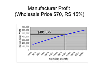
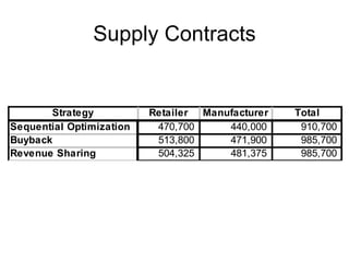
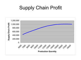
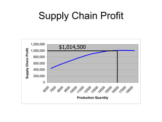
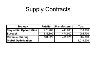
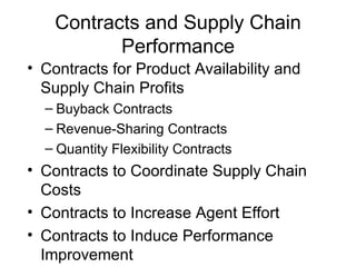
Inventory Management,
Supply Contracts and Risk
         Pooling

         Phil Kaminsky
        February 1, 2007
   kaminsky@ieor.berkeley.edu
Issues
• Inventory Management

• The Effect of Demand Uncertainty
  –   (s,S) Policy
  –   Periodic Review Policy
  –   Supply Contracts
  –   Risk Pooling

• Centralized vs. Decentralized Systems

• Practical Issues in Inventory Management
Customers,
                                     Field             demand
         Sources:      Regional      Warehouses:       centers
         plants        Warehouses:   stocking          sinks
         vendors       stocking      points
         ports         points


Supply


                       Inventory &
                       warehousing
                       costs
         Production/
         purchase      Transportation              Transportation
         costs         costs                       costs
                                    Inventory &
                                    warehousing
                                    costs
Inventory
• Where do we hold inventory?
   – Suppliers and manufacturers
   – warehouses and distribution centers
   – retailers
• Types of Inventory
   – WIP
   – raw materials
   – finished goods
• Why do we hold inventory?
   – Economies of scale
   – Uncertainty in supply and demand
   – Lead Time, Capacity limitations
Goals:
     Reduce Cost, Improve Service
• By effectively managing inventory:
  – Xerox eliminated $700 million inventory from
    its supply chain
  – Wal-Mart became the largest retail company
    utilizing efficient inventory management
  – GM has reduced parts inventory and
    transportation costs by 26% annually
Goals:
     Reduce Cost, Improve Service
• By not managing inventory successfully
  – In 1994, “IBM continues to struggle with shortages in
    their ThinkPad line” (WSJ, Oct 7, 1994)
  – In 1993, “Liz Claiborne said its unexpected earning
    decline is the consequence of higher than anticipated
    excess inventory” (WSJ, July 15, 1993)
  – In 1993, “Dell Computers predicts a loss; Stock
    plunges. Dell acknowledged that the company was
    sharply off in its forecast of demand, resulting in
    inventory write downs” (WSJ, August 1993)
Understanding Inventory
• The inventory policy is affected by:
  – Demand Characteristics
  – Lead Time
  – Number of Products
  – Objectives
     • Service level
     • Minimize costs
  – Cost Structure
Cost Structure
• Order costs
  – Fixed
  – Variable
• Holding Costs
  – Insurance
  – Maintenance and Handling
  – Taxes
  – Opportunity Costs
  – Obsolescence
EOQ: A Simple Model*
• Book Store Mug Sales
  – Demand is constant, at 20 units a week
  – Fixed order cost of $12.00, no lead time
  – Holding cost of 25% of inventory value
    annually
  – Mugs cost $1.00, sell for $5.00
• Question
  – How many, when to order?
EOQ: A View of Inventory*

               Note:
               • No Stockouts
               • Order when no inventory
               • Order Size determines policy
   Inventory


Order
Size

                                                  Avg. Inven

                                                Time
EOQ: Calculating Total Cost*
• Purchase Cost Constant
• Holding Cost: (Avg. Inven) * (Holding
  Cost)
• Ordering (Setup Cost):
     Number of Orders * Order Cost
• Goal: Find the Order Quantity that
          Minimizes These Costs:
EOQ:Total Cost*

       160
       140
       120          Total Cost
       100
Cost


                                       Holding Cost
       80
       60
       40                        Order Cost
       20
        0
             0         500          1000         1500
                        Order Quantity
EOQ: Optimal Order Quantity*
• Optimal Quantity =

 (2*Demand*Setup Cost)/holding cost

• So for our problem, the optimal quantity is
  316
EOQ: Important Observations*
• Tradeoff between set-up costs and holding
  costs when determining order quantity. In fact,
  we order so that these costs are equal per unit
  time
• Total Cost is not particularly sensitive to the
  optimal order quantity

Order Quantity 50%   80%   90%   100% 110% 120% 150% 200%
Cost Increase   125% 103% 101% 100% 101% 102% 108% 125%
The Effect of
         Demand Uncertainty
• Most companies treat the world as if it were
  predictable:
  – Production and inventory planning are based on
    forecasts of demand made far in advance of the
    selling season
  – Companies are aware of demand uncertainty when
    they create a forecast, but they design their planning
    process as if the forecast truly represents reality
• Recent technological advances have increased
  the level of demand uncertainty:
  – Short product life cycles
  – Increasing product variety
Demand Forecast
• The three principles of all forecasting
  techniques:

  – Forecasting is always wrong
  – The longer the forecast horizon the worst is
    the forecast
  – Aggregate forecasts are more accurate
SnowTime Sporting Goods
• Fashion items have short life cycles, high variety
  of competitors
• SnowTime Sporting Goods
  – New designs are completed
  – One production opportunity
  – Based on past sales, knowledge of the industry, and
    economic conditions, the marketing department has a
    probabilistic forecast
  – The forecast averages about 13,000, but there is a
    chance that demand will be greater or less than this.
Supply Chain Time Lines

         Jan 00                          Jan 01                    Jan 02
                       Design              Production            Retailing

              Feb 00            Sep 00       Feb 01     Sep 01
Production
SnowTime Demand Scenarios

                            Demand Scenarios
   Probability


                 30%
                 25%
                 20%
                 15%
                 10%
                  5%
                  0%
                                0


                                                0


                                                        0
                                        0


                                                                0
                       00

                             00


                                             00


                                                     00
                                     00


                                                             00
                  80

                            10


                                    12


                                            14


                                                    16


                                                            18
                                             Sales
SnowTime Costs
•   Production cost per unit (C): $80
•   Selling price per unit (S): $125
•   Salvage value per unit (V): $20
•   Fixed production cost (F): $100,000
•   Q is production quantity, D demand

• Profit =
  Revenue - Variable Cost - Fixed Cost + Salvage
SnowTime Scenarios
• Scenario One:
  – Suppose you make 12,000 jackets and demand ends
    up being 13,000 jackets.
  – Profit = 125(12,000) - 80(12,000) - 100,000 =
    $440,000
• Scenario Two:
  – Suppose you make 12,000 jackets and demand ends
    up being 11,000 jackets.
  – Profit = 125(11,000) - 80(12,000) - 100,000 +
    20(1000) = $ 335,000
SnowTime Best Solution
• Find order quantity that maximizes
  weighted average profit.
• Question: Will this quantity be less than,
  equal to, or greater than average
  demand?
What to Make?
• Question: Will this quantity be less than,
  equal to, or greater than average
  demand?
• Average demand is 13,100
• Look at marginal cost Vs. marginal profit
  – if extra jacket sold, profit is 125-80 = 45
  – if not sold, cost is 80-20 = 60
• So we will make less than average
SnowTime Expected Profit

                      Expected Profit

         $400,000

         $300,000
Profit


         $200,000

         $100,000

              $0
               8000       12000      16000   20000
                            Order Quantity
SnowTime Expected Profit
                       Expected Profit

          $400,000

          $300,000
 Profit


          $200,000

          $100,000

               $0
                8000       12000      16000   20000
                             Order Quantity
SnowTime:
      Important Observations
• Tradeoff between ordering enough to meet
  demand and ordering too much
• Several quantities have the same average profit
• Average profit does not tell the whole story

• Question: 9000 and 16000 units
  lead to about the same average
  profit, so which do we prefer?
SnowTime Expected Profit

                      Expected Profit

         $400,000

         $300,000
Profit


         $200,000

         $100,000

              $0
               8000       12000      16000   20000
                            Order Quantity
Probability of Outcomes
              100%
              80%
Probability


              60%              Q=9000
              40%              Q=16000

              20%
               0%
                      0

                      0

                    00

                    00

                    00
                   00
                   00


                  00

                  00

                  00
                 00
                 00


               10

               30

               50
              -3

              -1


                     Revenue
Key Insights from this Model
• The optimal order quantity is not necessarily
  equal to average forecast demand
• The optimal quantity depends on the relationship
  between marginal profit and marginal cost
• As order quantity increases, average profit first
  increases and then decreases
• As production quantity increases, risk increases.
   In other words, the probability of large gains and
  of large losses increases
SnowTime Costs: Initial
              Inventory
•   Production cost per unit (C): $80
•   Selling price per unit (S): $125
•   Salvage value per unit (V): $20
•   Fixed production cost (F): $100,000
•   Q is production quantity, D demand


• Profit =
    Revenue - Variable Cost - Fixed Cost +
    Salvage
SnowTime Expected Profit

                      Expected Profit

         $400,000

         $300,000
Profit


         $200,000

         $100,000

              $0
               8000       12000      16000   20000
                            Order Quantity
Initial Inventory
• Suppose that one of the jacket designs is a
  model produced last year.
• Some inventory is left from last year
• Assume the same demand pattern as before
• If only old inventory is sold, no setup cost

• Question: If there are 7000 units remaining, what
  should SnowTime do? What should they do if
  there are 10,000 remaining?
Initial Inventory and Profit


         500000
         400000
         300000
Profit


         200000
         100000
              0
                  00

                       00

                            00
            00


                                  0


                                             0

                                                   0
                                       0
                                 00


                                           00

                                                  50
                                      50
           50

                  65

                       80

                            95
                                 11

                                      12

                                           14

                                                  15
                            Production Quantity
Initial Inventory and Profit

         500000
         400000
         300000
Profit


         200000
         100000
              0
                  6000
                  5000

                         7000
                                8000
                                9000
                                       10000
                                       11000
                                               12000
                                                       13000
                                                       14000
                                                               15000
                                                               16000
                                Production Quantity
Supply Contracts

Fixed Production Cost =$100,000

Variable Production Cost=$35

                               Wholesale Price =$80

                                                            Selling Price=$125
                                                            Salvage Value=$20


 Manufacturer          Manufacturer DC          Retail DC


                                                                    Stores
Demand Scenarios

                    Demand Scenarios

              30%
Probability


              25%
              20%
              15%
              10%
               5%
               0%
                  00


                   0
                   0

                   0

                   0

                   0
                 00

                 00

                 00

                 00

                 00
                80

               10


               18
               12

               14

               16


                              Sales
Distributor Expected Profit

                     Expected Profit

500000

400000

300000

200000

100000

    0
    6000   8000   10000   12000   14000    16000   18000   20000
                          Order Quantity
Distributor Expected Profit

                     Expected Profit

500000

400000

300000

200000

100000

    0
    6000   8000   10000   12000   14000    16000   18000   20000
                          Order Quantity
Supply Contracts (cont.)
• Distributor optimal order quantity is 12,000
  units
• Distributor expected profit is $470,000
• Manufacturer profit is $440,000
• Supply Chain Profit is $910,000

    –Is there anything that the distributor and
    manufacturer can do to increase the profit
    of both?
Supply Contracts

Fixed Production Cost =$100,000

Variable Production Cost=$35

                                  Wholesale Price =$80

                                                              Selling Price=$125
                                                              Salvage Value=$20


 Manufacturer          Manufacturer DC            Retail DC


                                                                      Stores
Retailer Profit
                            (Buy Back=$55)
                  600,000
                  500,000
Retailer Profit


                  400,000
                  300,000
                  200,000

                  100,000
                       0
                          00

                          00

                          00

                          00


                           0

                           0


                           0


                           0
                           0


                           0


                           0

                           0


                           0
                         00

                         00

                         00

                         00

                         00

                         00

                         00

                         00

                         00
                        60


                        80

                        90
                        70


                       11

                       12

                       13

                       14


                       17

                       18
                       10


                       15

                       16
                                  Order Quantity
Retailer Profit
                            (Buy Back=$55)
                  600,000
                            $513,800
                  500,000
Retailer Profit


                  400,000
                  300,000
                  200,000

                  100,000
                       0
                          00

                          00

                          00

                          00


                           0

                           0


                           0


                           0
                           0


                           0


                           0

                           0


                           0
                         00

                         00

                         00

                         00

                         00

                         00

                         00

                         00

                         00
                        60


                        80

                        90
                        70


                       11

                       12

                       13

                       14


                       17

                       18
                       10


                       15

                       16
                                       Order Quantity
Manufacturer Profit
                       (Buy Back=$55)

                      600,000
Manufacturer Profit


                      500,000

                      400,000

                      300,000
                      200,000

                      100,000

                           0
                              00


                              00
                              00


                              00

                               0

                               0

                               0

                               0

                               0

                               0

                               0

                               0

                               0
                             00

                             00

                             00

                             00

                             00

                             00

                             00

                             00

                             00
                            60

                            70

                            80

                            90
                           10

                           11


                           13


                           16

                           17

                           18
                           12


                           14

                           15
                                Production Quantity
Manufacturer Profit
                       (Buy Back=$55)

                      600,000
                                $471,900
Manufacturer Profit


                      500,000

                      400,000

                      300,000
                      200,000

                      100,000

                           0
                              00


                              00
                              00


                              00

                               0

                               0

                               0

                               0

                               0

                               0

                               0

                               0

                               0
                             00

                             00

                             00

                             00

                             00

                             00

                             00

                             00

                             00
                            60

                            70

                            80

                            90
                           10

                           11


                           13


                           16

                           17

                           18
                           12


                           14

                           15
                                      Production Quantity
Supply Contracts

Fixed Production Cost =$100,000

Variable Production Cost=$35

                                  Wholesale Price =$??

                                                              Selling Price=$125
                                                              Salvage Value=$20


 Manufacturer          Manufacturer DC            Retail DC


                                                                      Stores
Retailer Profit
(Wholesale Price $70, RS 15%)

                  600,000
                  500,000
Retailer Profit


                  400,000
                  300,000
                  200,000
                  100,000
                       0
                          00

                          00


                           0
                          00


                          00

                           0

                           0

                           0

                           0

                           0

                           0

                           0


                           0
                         00

                         00

                         00


                         00

                         00

                         00

                         00

                         00
                         00
                        70
                        60


                        80

                        90
                       10


                       14

                       15


                       17

                       18
                       11

                       12

                       13


                       16
                            Order Quantity
Retailer Profit
(Wholesale Price $70, RS 15%)

                  600,000
                            $504,325
                  500,000
Retailer Profit


                  400,000
                  300,000
                  200,000
                  100,000
                       0
                          00

                          00


                           0
                          00


                          00

                           0

                           0

                           0

                           0

                           0

                           0

                           0


                           0
                         00

                         00

                         00


                         00

                         00

                         00

                         00

                         00
                         00
                        70
                        60


                        80

                        90
                       10


                       14

                       15


                       17

                       18
                       11

                       12

                       13


                       16
                                   Order Quantity
Manufacturer Profit
(Wholesale Price $70, RS 15%)

                       700,000
                       600,000
 Manufacturer Profit


                       500,000
                       400,000
                       300,000
                       200,000
                       100,000
                            0
                               00

                               00

                               00

                               00

                                0

                                0

                                0

                                0

                                0

                                0

                                0

                                0

                                0
                              00


                              00
                              00

                              00

                              00

                              00

                              00


                              00


                              00
                             60

                             70


                             90
                             80


                            11

                            12

                            13

                            14

                            15


                            17
                            10


                            16


                            18
                                 Production Quantity
Manufacturer Profit
(Wholesale Price $70, RS 15%)

                       700,000
                       600,000
 Manufacturer Profit


                       500,000   $481,375
                       400,000
                       300,000
                       200,000
                       100,000
                            0
                               00

                               00

                               00

                               00

                                0

                                0

                                0

                                0

                                0

                                0

                                0

                                0

                                0
                              00


                              00
                              00

                              00

                              00

                              00

                              00


                              00


                              00
                             60

                             70


                             90
                             80


                            11

                            12

                            13

                            14

                            15


                            17
                            10


                            16


                            18
                                       Production Quantity
Supply Contracts


       Strategy           Retailer Manufacturer   Total
Sequential Optimization    470,700     440,000     910,700
Buyback                    513,800     471,900     985,700
Revenue Sharing            504,325     481,375     985,700
Supply Contracts

Fixed Production Cost =$100,000

Variable Production Cost=$35

                               Wholesale Price =$80

                                                            Selling Price=$125
                                                            Salvage Value=$20


 Manufacturer          Manufacturer DC          Retail DC


                                                                    Stores
Supply Chain Profit

                      1,200,000
Supply Chain Profit


                      1,000,000
                       800,000

                       600,000
                       400,000

                       200,000
                             0
                                0

                                0

                                0


                                0

                                0

                                0

                                0

                                0
                               00

                               00

                               00

                               00


                                0
                              00


                              00


                              00
                              00


                              00

                              00


                              00

                              00


                              00
                             60

                             70

                             80

                             90
                            10

                            11

                            12


                            14

                            15

                            16

                            17

                            18
                            13


                                          Production Quantity
Supply Chain Profit

                      1,200,000
                                  $1,014,500
Supply Chain Profit


                      1,000,000
                       800,000

                       600,000
                       400,000
                       200,000
                             0
                               00


                               00


                                0


                                0

                                0
                               00


                               00

                                0


                                0


                                0

                                0

                                0

                                0
                              00


                              00
                              00


                              00


                              00

                              00

                              00

                              00

                              00
                             60

                             70

                             80

                             90
                            10

                            11

                            12

                            13

                            14

                            15

                            16

                            17

                            18
                                        Production Quantity
Supply Contracts

        Strategy          Retailer Manufacturer   Total
Sequential Optimization    470,700     440,000      910,700
Buyback                    513,800     471,900      985,700
Revenue Sharing            504,325     481,375      985,700
Global Optimization                               1,014,500
Supply Contracts: Key Insights
• Effective supply contracts allow supply
  chain partners to replace sequential
  optimization by global optimization
• Buy Back and Revenue Sharing contracts
  achieve this objective through risk
  sharing
Contracts and Supply Chain
           Performance
• Contracts for Product Availability and
  Supply Chain Profits
  – Buyback Contracts
  – Revenue-Sharing Contracts
  – Quantity Flexibility Contracts
• Contracts to Coordinate Supply Chain
  Costs
• Contracts to Increase Agent Effort
• Contracts to Induce Performance
  Improvement
Contracts for Product Availability
     and Supply Chain Profits
• Many shortcomings in supply chain performance occur
  because the buyer and supplier are separate
  organizations and each tries to optimize its own profit
• Total supply chain profits might therefore be lower than if
  the supply chain coordinated actions to have a common
  objective of maximizing total supply chain profits
• Double marginalization results in suboptimal order
  quantity
• An approach to dealing with this problem is to design a
  contract that encourages a buyer to purchase more and
  increase the level of product availability
• The supplier must share in some of the buyer’s demand
  uncertainty, however
Contracts for Product Availability and
Supply Chain Profits: Buyback Contracts
• Allows a retailer to return unsold inventory up to a
  specified amount at an agreed upon price
• Increases the optimal order quantity for the retailer,
  resulting in higher product availability and higher profits
  for both the retailer and the supplier
• Most effective for products with low variable cost, such as
  music, software, books, magazines, and newspapers
• Downside is that buyback contract results in surplus
  inventory that must be disposed of, which increases
  supply chain costs
• Can also increase information distortion through the
  supply chain because the supply chain reacts to retail
  orders, not actual customer demand
Contracts for Product Availability and Supply
 Chain Profits: Revenue Sharing Contracts

• The buyer pays a minimal amount for each
  unit purchased from the supplier but
  shares a fraction of the revenue for each
  unit sold
• Decreases the cost per unit charged to the
  retailer, which effectively decreases the
  cost of overstocking
• Can result in supply chain information
  distortion, however, just as in the case of
  buyback contracts
Contracts for Product Availability and
Supply Chain Profits: Quantity Flexibility
               Contracts
• Allows the buyer to modify the order
  (within limits) as demand visibility
  increases closer to the point of sale
• Better matching of supply and demand
• Increased overall supply chain profits if the
  supplier has flexible capacity
• Lower levels of information distortion than
  either buyback contracts or revenue
  sharing contracts
Contracts to Coordinate
       Supply Chain Costs
• Differences in costs at the buyer and supplier
  can lead to decisions that increase total supply
  chain costs
• Example: Replenishment order size placed by
  the buyer. The buyer’s EOQ does not take into
  account the supplier’s costs.
• A quantity discount contract may encourage the
  buyer to purchase a larger quantity (which would
  be lower costs for the supplier), which would
  result in lower total supply chain costs
• Quantity discounts lead to information distortion
  because of order batching
Contracts to Increase Agent
              Effort
• There are many instances in a supply chain
  where an agent acts on the behalf of a principal
  and the agent’s actions affect the reward for the
  principal
• Example: A car dealer who sells the cars of a
  manufacturer, as well as those of other
  manufacturers
• Examples of contracts to increase agent effort
  include two-part tariffs and threshold contracts
• Threshold contracts increase information
  distortion, however
Contracts to Induce
    Performance Improvement
• A buyer may want performance improvement
  from a supplier who otherwise would have little
  incentive to do so
• A shared savings contract provides the supplier
  with
  a fraction of the savings that result from the
  performance improvement
• Particularly effective where the benefit from
  improvement accrues primarily to the buyer, but
  where the effort for the improvement comes
  primarily from the supplier
Supply Contracts: Case Study
• Example: Demand for a movie newly released
  video cassette typically starts high and
  decreases rapidly
  – Peak demand last about 10 weeks
• Blockbuster purchases a copy from a studio for
  $65 and rent for $3
  – Hence, retailer must rent the tape at least 22 times
    before earning profit
• Retailers cannot justify purchasing enough to
  cover the peak demand
  – In 1998, 20% of surveyed customers reported that
    they could not rent the movie they wanted
Supply Contracts: Case Study
• Starting in 1998 Blockbuster entered a revenue
  sharing agreement with the major studios
  – Studio charges $8 per copy
  – Blockbuster pays 30-45% of its rental income
• Even if Blockbuster keeps only half of the rental
  income, the breakeven point is 6 rental per copy
• The impact of revenue sharing on Blockbuster
  was dramatic
  – Rentals increased by 75% in test markets
  – Market share increased from 25% to 31% (The 2nd
    largest retailer, Hollywood Entertainment Corp has
    5% market share)
(s, S) Policies
• For some starting inventory levels, it is better to
  not start production
• If we start, we always produce to the same level
• Thus, we use an (s,S) policy. If the inventory
  level is below s, we produce up to S.
• s is the reorder point, and S is the order-up-to
  level
• The difference between the two levels is driven
  by the fixed costs associated with ordering,
  transportation, or manufacturing
A Multi-Period Inventory Model

• Often, there are multiple reorder
  opportunities

• Consider a central distribution facility
  which orders from a manufacturer and
  delivers to retailers. The distributor
  periodically places orders to replenish its
  inventory
Reminder:
    The Normal Distribution

                               Standard Deviation = 5

Standard Deviation = 10


                     Average = 30

0      10       20        30        40      50          60
The DC holds inventory to:

• Satisfy demand during lead
  time
• Protect against demand
  uncertainty
• Balance fixed costs and
  holding costs
The Multi-Period Continuous
      Review Inventory Model
• Normally distributed random demand
• Fixed order cost plus a cost proportional to
  amount ordered.
• Inventory cost is charged per item per unit time
• If an order arrives and there is no inventory, the
  order is lost
• The distributor has a required service level. This
  is expressed as the the likelihood that the
  distributor will not stock out during lead time.
• Intuitively, how will this effect our policy?
A View of (s, S) Policy

                  S
                                       Inventory Position
Inventory Level


                                Lead
                                Time

                  s


                  0
                                                Time
The (s,S) Policy
• (s, S) Policy: Whenever the inventory
  position drops below a certain level, s, we
  order to raise the inventory position to
  level S.
• The reorder point is a function of:
  – The Lead Time
  – Average demand
  – Demand variability
  – Service level
Notation
• AVG = average daily demand
• STD = standard deviation of daily demand
• LT = replenishment lead time in days
• h = holding cost of one unit for one day
• K = fixed cost
• SL = service level (for example, 95%). This implies that
  the probability of stocking out is 100%-SL (for example,
  5%)
• Also, the Inventory Position at any time is the actual
  inventory plus items already ordered, but not yet
  delivered.
Analysis
• The reorder point (s) has two components:
   – To account for average demand during lead time:
                        LT×AVG
   – To account for deviations from average (we call this safety
     stock)
                        z × STD × √LT
     where z is chosen from statistical tables to ensure that the
     probability of stockouts during leadtime is 100%-SL.

• Since there is a fixed cost, we order more than up to the
  reorder point:
             Q=√(2 ×K ×AVG)/h
• The total order-up-to level is:
                         S=Q+s
Example
• The distributor has historically observed weekly demand
  of:
      AVG = 44.6 STD = 32.1
  Replenishment lead time is 2 weeks, and desired service
  level SL = 97%
• Average demand during lead time is:
      44.6 × 2 = 89.2
• Safety Stock is:
      1.88 × 32.1 × √2 = 85.3
• Reorder point is thus 175, or about 3.9 = (175/44.6)
  weeks of supply at warehouse and in the pipeline
Example, Cont.
• Weekly inventory holding cost: 0.87=
  (0.18x250/52)
  – Therefore, Q=679
• Order-up-to level thus equals:
  – Reorder Point + Q = 176+679 = 855
Periodic Review
• Suppose the distributor places
  orders every month
• What policy should the distributor
  use?
• What about the fixed cost?
Base-Stock Policy

                                       r                   r


                                   L                   L          L
                  Base-stock
                  Level                    Inventory
Inventory Level


                                            Position


                         0
                                                           Time
Periodic Review Policy
• Each review echelon, inventory position is
  raised to the base-stock level.
• The base-stock level includes two
  components:
  – Average demand during r+L days (the time
    until the next order arrives):
                  (r+L)*AVG
  – Safety stock during that time:
            z*STD* √r+L
Risk Pooling
• Consider these two systems:
             Warehouse One      Market One
Supplier
             Warehouse Two      Market Two


                                 Market One
 Supplier      Warehouse

                                 Market Two
Risk Pooling
• For the same service level, which system
  will require more inventory? Why?
• For the same total inventory level, which
  system will have better service? Why?
• What are the factors that affect these
  answers?
Risk Pooling Example
• Compare the two systems:
  – two products
  – maintain 97% service level
  – $60 order cost
  – $.27 weekly holding cost
  – $1.05 transportation cost per unit in
    decentralized system, $1.10 in centralized
    system
  – 1 week lead time
Risk Pooling Example


Week         1    2    3    4    5    6    7    8
Prod A,      33   45   37   38   55   30   18   58
Market 1
Prod A,      46   35   41   40   26   48   18   55
Market 2
Prod B,      0    2    3    0    0    1    3    0
Market 1
Product B,   2    4    0    0    3    1    0    0
Market 2
Risk Pooling Example
Warehouse Product AVG    STD    CV

Market 1   A     39.3    13.2   .34


Market 2   A     38.6    12.0   .31


Market 1   B     1.125   1.36   1.21


Market 2   B     1.25    1.58   1.26
Risk Pooling Example
Warehouse Product AVG   STD CV     s    S     Avg. %
                                              Inven. Dec.
Market 1   A    39.3    13.2 .34   65   197   91
Market 2   A    38.6    12.0 .31   62   193   88
Market 1   B    1.125 1.36 1.21 4       29    14
Market 2   B    1.25 1.58 1.26 5        29    15
Cent.      A    77.9 20.7 .27      118 304    132    36%
Cent       B    2.375 1.9 .81      6   39     20     43%
Risk Pooling:
      Important Observations
• Centralizing inventory control reduces
  both safety stock and average inventory
  level for the same service level.
• This works best for
  – High coefficient of variation, which increases
    required safety stock.
  – Negatively correlated demand. Why?
• What other kinds of risk pooling will we
  see?
To Centralize or not to Centralize
• What is the effect on:
  – Safety stock?
  – Service level?
  – Overhead?
  – Lead time?
  – Transportation Costs?
Centralized Systems*

                         Supplier


                    Warehouse


                               Retailers

• Centralized Decision
Centralized Distribution
             Systems*
• Question: How much inventory should management
  keep at each location?
• A good strategy:
   – The retailer raises inventory to level Sr each period
   – The supplier raises the sum of inventory in the
     retailer and supplier warehouses and in transit to
     Ss
   – If there is not enough inventory in the warehouse
     to meet all demands from retailers, it is allocated
     so that the service level at each of the retailers will
     be equal.
Inventory Management: Best
              Practice
• Periodic inventory reviews
• Tight management of usage rates, lead
  times and safety stock
• ABC approach
• Reduced safety stock levels
• Shift more inventory, or inventory
  ownership, to suppliers
• Quantitative approaches
Changes In Inventory Turnover
• Inventory turnover ratio =
        annual sales/avg. inventory level
• Inventory turns increased by 30% from
  1995 to 1998
• Inventory turns increased by 27% from
  1998 to 2000
• Overall the increase is from 8.0 turns per
  year to over 13 per year over a five year
  period ending in year 2000.
Inventory Turnover Ratio
     Industry           Upper     Median   Lower
                       Quartile            Quartile
   Dairy Products        34.4      19.3      9.2
Electronic Component     9.8       5.7       3.7
Electronic Computers     9.4       5.3       3.5
 Books: publishing       9.8       2.4       1.3

Household audio &        6.2       3.4       2.3
 video equipment
Household electrical     8.0       5.0       3.8
    appliances
Industrial chemical     10.3       6.6       4.4
Factors that Drive Reduction in
           Inventory
• Top management emphasis on inventory
  reduction (19%)
• Reduce the Number of SKUs in the warehouse
  (10%)
• Improved forecasting (7%)
• Use of sophisticated inventory management
  software (6%)
• Coordination among supply chain members
  (6%)
• Others
Factors that Drive Inventory Turns
                Increase
• Better software for inventory management
  (16.2%)
• Reduced lead time (15%)
• Improved forecasting (10.7%)
• Application of SCM principals (9.6%)
• More attention to inventory management (6.6%)
• Reduction in SKU (5.1%)
• Others
Forecasting
• Recall the three rules
• Nevertheless, forecast is critical
• General Overview:
  – Judgment methods
  – Market research methods
  – Time Series methods
  – Causal methods
Judgment Methods
• Assemble the opinion of experts
• Sales-force composite combines
  salespeople’s estimates
• Panels of experts – internal, external, both
• Delphi method
  – Each member surveyed
  – Opinions are compiled
  – Each member is given the opportunity to
    change his opinion
Market Research Methods
• Particularly valuable for developing
  forecasts of newly introduced products
• Market testing
  – Focus groups assembled.
  – Responses tested.
  – Extrapolations to rest of market made.
• Market surveys
  – Data gathered from potential customers
  – Interviews, phone-surveys, written surveys,
    etc.
Time Series Methods
• Past data is used to estimate future data
• Examples include
   – Moving averages – average of some previous demand points.
   – Exponential Smoothing – more recent points receive more
     weight
   – Methods for data with trends:
      • Regression analysis – fits line to data
      • Holt’s method – combines exponential smoothing concepts with the
        ability to follow a trend
   – Methods for data with seasonality
      • Seasonal decomposition methods (seasonal patterns removed)
      • Winter’s method: advanced approach based on exponential
        smoothing
   – Complex methods (not clear that these work better)
Causal Methods
• Forecasts are generated based on data
  other than the data being predicted
• Examples include:
  – Inflation rates
  – GNP
  – Unemployment rates
  – Weather
  – Sales of other products
Selecting the Appropriate
                 Approach:
• What is the purpose of the forecast?
   – Gross or detailed estimates?
• What are the dynamics of the system being forecast?
   – Is it sensitive to economic data?
   – Is it seasonal? Trending?
• How important is the past in estimating the future?
• Different approaches may be appropriate for different
  stages of the product lifecycle:
   – Testing and intro: market research methods, judgment methods
   – Rapid growth: time series methods
   – Mature: time series, causal methods (particularly for long-range
     planning)
• It is typically effective to combine approaches.

Inventory management-1224844053656038-9

  • 1.
    Inventory Management, Supply Contractsand Risk Pooling Phil Kaminsky February 1, 2007 kaminsky@ieor.berkeley.edu
  • 2.
    Issues • Inventory Management •The Effect of Demand Uncertainty – (s,S) Policy – Periodic Review Policy – Supply Contracts – Risk Pooling • Centralized vs. Decentralized Systems • Practical Issues in Inventory Management
  • 3.
    Customers, Field demand Sources: Regional Warehouses: centers plants Warehouses: stocking sinks vendors stocking points ports points Supply Inventory & warehousing costs Production/ purchase Transportation Transportation costs costs costs Inventory & warehousing costs
  • 4.
    Inventory • Where dowe hold inventory? – Suppliers and manufacturers – warehouses and distribution centers – retailers • Types of Inventory – WIP – raw materials – finished goods • Why do we hold inventory? – Economies of scale – Uncertainty in supply and demand – Lead Time, Capacity limitations
  • 5.
    Goals: Reduce Cost, Improve Service • By effectively managing inventory: – Xerox eliminated $700 million inventory from its supply chain – Wal-Mart became the largest retail company utilizing efficient inventory management – GM has reduced parts inventory and transportation costs by 26% annually
  • 6.
    Goals: Reduce Cost, Improve Service • By not managing inventory successfully – In 1994, “IBM continues to struggle with shortages in their ThinkPad line” (WSJ, Oct 7, 1994) – In 1993, “Liz Claiborne said its unexpected earning decline is the consequence of higher than anticipated excess inventory” (WSJ, July 15, 1993) – In 1993, “Dell Computers predicts a loss; Stock plunges. Dell acknowledged that the company was sharply off in its forecast of demand, resulting in inventory write downs” (WSJ, August 1993)
  • 7.
    Understanding Inventory • Theinventory policy is affected by: – Demand Characteristics – Lead Time – Number of Products – Objectives • Service level • Minimize costs – Cost Structure
  • 8.
    Cost Structure • Ordercosts – Fixed – Variable • Holding Costs – Insurance – Maintenance and Handling – Taxes – Opportunity Costs – Obsolescence
  • 9.
    EOQ: A SimpleModel* • Book Store Mug Sales – Demand is constant, at 20 units a week – Fixed order cost of $12.00, no lead time – Holding cost of 25% of inventory value annually – Mugs cost $1.00, sell for $5.00 • Question – How many, when to order?
  • 10.
    EOQ: A Viewof Inventory* Note: • No Stockouts • Order when no inventory • Order Size determines policy Inventory Order Size Avg. Inven Time
  • 11.
    EOQ: Calculating TotalCost* • Purchase Cost Constant • Holding Cost: (Avg. Inven) * (Holding Cost) • Ordering (Setup Cost): Number of Orders * Order Cost • Goal: Find the Order Quantity that Minimizes These Costs:
  • 12.
    EOQ:Total Cost* 160 140 120 Total Cost 100 Cost Holding Cost 80 60 40 Order Cost 20 0 0 500 1000 1500 Order Quantity
  • 13.
    EOQ: Optimal OrderQuantity* • Optimal Quantity = (2*Demand*Setup Cost)/holding cost • So for our problem, the optimal quantity is 316
  • 14.
    EOQ: Important Observations* •Tradeoff between set-up costs and holding costs when determining order quantity. In fact, we order so that these costs are equal per unit time • Total Cost is not particularly sensitive to the optimal order quantity Order Quantity 50% 80% 90% 100% 110% 120% 150% 200% Cost Increase 125% 103% 101% 100% 101% 102% 108% 125%
  • 15.
    The Effect of Demand Uncertainty • Most companies treat the world as if it were predictable: – Production and inventory planning are based on forecasts of demand made far in advance of the selling season – Companies are aware of demand uncertainty when they create a forecast, but they design their planning process as if the forecast truly represents reality • Recent technological advances have increased the level of demand uncertainty: – Short product life cycles – Increasing product variety
  • 16.
    Demand Forecast • Thethree principles of all forecasting techniques: – Forecasting is always wrong – The longer the forecast horizon the worst is the forecast – Aggregate forecasts are more accurate
  • 17.
    SnowTime Sporting Goods •Fashion items have short life cycles, high variety of competitors • SnowTime Sporting Goods – New designs are completed – One production opportunity – Based on past sales, knowledge of the industry, and economic conditions, the marketing department has a probabilistic forecast – The forecast averages about 13,000, but there is a chance that demand will be greater or less than this.
  • 18.
    Supply Chain TimeLines Jan 00 Jan 01 Jan 02 Design Production Retailing Feb 00 Sep 00 Feb 01 Sep 01 Production
  • 19.
    SnowTime Demand Scenarios Demand Scenarios Probability 30% 25% 20% 15% 10% 5% 0% 0 0 0 0 0 00 00 00 00 00 00 80 10 12 14 16 18 Sales
  • 20.
    SnowTime Costs • Production cost per unit (C): $80 • Selling price per unit (S): $125 • Salvage value per unit (V): $20 • Fixed production cost (F): $100,000 • Q is production quantity, D demand • Profit = Revenue - Variable Cost - Fixed Cost + Salvage
  • 21.
    SnowTime Scenarios • ScenarioOne: – Suppose you make 12,000 jackets and demand ends up being 13,000 jackets. – Profit = 125(12,000) - 80(12,000) - 100,000 = $440,000 • Scenario Two: – Suppose you make 12,000 jackets and demand ends up being 11,000 jackets. – Profit = 125(11,000) - 80(12,000) - 100,000 + 20(1000) = $ 335,000
  • 22.
    SnowTime Best Solution •Find order quantity that maximizes weighted average profit. • Question: Will this quantity be less than, equal to, or greater than average demand?
  • 23.
    What to Make? •Question: Will this quantity be less than, equal to, or greater than average demand? • Average demand is 13,100 • Look at marginal cost Vs. marginal profit – if extra jacket sold, profit is 125-80 = 45 – if not sold, cost is 80-20 = 60 • So we will make less than average
  • 24.
    SnowTime Expected Profit Expected Profit $400,000 $300,000 Profit $200,000 $100,000 $0 8000 12000 16000 20000 Order Quantity
  • 25.
    SnowTime Expected Profit Expected Profit $400,000 $300,000 Profit $200,000 $100,000 $0 8000 12000 16000 20000 Order Quantity
  • 26.
    SnowTime: Important Observations • Tradeoff between ordering enough to meet demand and ordering too much • Several quantities have the same average profit • Average profit does not tell the whole story • Question: 9000 and 16000 units lead to about the same average profit, so which do we prefer?
  • 27.
    SnowTime Expected Profit Expected Profit $400,000 $300,000 Profit $200,000 $100,000 $0 8000 12000 16000 20000 Order Quantity
  • 28.
    Probability of Outcomes 100% 80% Probability 60% Q=9000 40% Q=16000 20% 0% 0 0 00 00 00 00 00 00 00 00 00 00 10 30 50 -3 -1 Revenue
  • 29.
    Key Insights fromthis Model • The optimal order quantity is not necessarily equal to average forecast demand • The optimal quantity depends on the relationship between marginal profit and marginal cost • As order quantity increases, average profit first increases and then decreases • As production quantity increases, risk increases. In other words, the probability of large gains and of large losses increases
  • 30.
    SnowTime Costs: Initial Inventory • Production cost per unit (C): $80 • Selling price per unit (S): $125 • Salvage value per unit (V): $20 • Fixed production cost (F): $100,000 • Q is production quantity, D demand • Profit = Revenue - Variable Cost - Fixed Cost + Salvage
  • 31.
    SnowTime Expected Profit Expected Profit $400,000 $300,000 Profit $200,000 $100,000 $0 8000 12000 16000 20000 Order Quantity
  • 32.
    Initial Inventory • Supposethat one of the jacket designs is a model produced last year. • Some inventory is left from last year • Assume the same demand pattern as before • If only old inventory is sold, no setup cost • Question: If there are 7000 units remaining, what should SnowTime do? What should they do if there are 10,000 remaining?
  • 33.
    Initial Inventory andProfit 500000 400000 300000 Profit 200000 100000 0 00 00 00 00 0 0 0 0 00 00 50 50 50 65 80 95 11 12 14 15 Production Quantity
  • 34.
    Initial Inventory andProfit 500000 400000 300000 Profit 200000 100000 0 00 00 00 00 0 0 0 0 00 00 50 50 50 65 80 95 11 12 14 15 Production Quantity
  • 35.
    Initial Inventory andProfit 500000 400000 300000 Profit 200000 100000 0 00 00 00 00 0 0 0 0 00 00 50 50 50 65 80 95 11 12 14 15 Production Quantity
  • 36.
    Initial Inventory andProfit 500000 400000 300000 Profit 200000 100000 0 6000 5000 7000 8000 9000 10000 11000 12000 13000 14000 15000 16000 Production Quantity
  • 37.
    Supply Contracts Fixed ProductionCost =$100,000 Variable Production Cost=$35 Wholesale Price =$80 Selling Price=$125 Salvage Value=$20 Manufacturer Manufacturer DC Retail DC Stores
  • 38.
    Demand Scenarios Demand Scenarios 30% Probability 25% 20% 15% 10% 5% 0% 00 0 0 0 0 0 00 00 00 00 00 80 10 18 12 14 16 Sales
  • 39.
    Distributor Expected Profit Expected Profit 500000 400000 300000 200000 100000 0 6000 8000 10000 12000 14000 16000 18000 20000 Order Quantity
  • 40.
    Distributor Expected Profit Expected Profit 500000 400000 300000 200000 100000 0 6000 8000 10000 12000 14000 16000 18000 20000 Order Quantity
  • 41.
    Supply Contracts (cont.) •Distributor optimal order quantity is 12,000 units • Distributor expected profit is $470,000 • Manufacturer profit is $440,000 • Supply Chain Profit is $910,000 –Is there anything that the distributor and manufacturer can do to increase the profit of both?
  • 42.
    Supply Contracts Fixed ProductionCost =$100,000 Variable Production Cost=$35 Wholesale Price =$80 Selling Price=$125 Salvage Value=$20 Manufacturer Manufacturer DC Retail DC Stores
  • 43.
    Retailer Profit (Buy Back=$55) 600,000 500,000 Retailer Profit 400,000 300,000 200,000 100,000 0 00 00 00 00 0 0 0 0 0 0 0 0 0 00 00 00 00 00 00 00 00 00 60 80 90 70 11 12 13 14 17 18 10 15 16 Order Quantity
  • 44.
    Retailer Profit (Buy Back=$55) 600,000 $513,800 500,000 Retailer Profit 400,000 300,000 200,000 100,000 0 00 00 00 00 0 0 0 0 0 0 0 0 0 00 00 00 00 00 00 00 00 00 60 80 90 70 11 12 13 14 17 18 10 15 16 Order Quantity
  • 45.
    Manufacturer Profit (Buy Back=$55) 600,000 Manufacturer Profit 500,000 400,000 300,000 200,000 100,000 0 00 00 00 00 0 0 0 0 0 0 0 0 0 00 00 00 00 00 00 00 00 00 60 70 80 90 10 11 13 16 17 18 12 14 15 Production Quantity
  • 46.
    Manufacturer Profit (Buy Back=$55) 600,000 $471,900 Manufacturer Profit 500,000 400,000 300,000 200,000 100,000 0 00 00 00 00 0 0 0 0 0 0 0 0 0 00 00 00 00 00 00 00 00 00 60 70 80 90 10 11 13 16 17 18 12 14 15 Production Quantity
  • 47.
    Supply Contracts Fixed ProductionCost =$100,000 Variable Production Cost=$35 Wholesale Price =$?? Selling Price=$125 Salvage Value=$20 Manufacturer Manufacturer DC Retail DC Stores
  • 48.
    Retailer Profit (Wholesale Price$70, RS 15%) 600,000 500,000 Retailer Profit 400,000 300,000 200,000 100,000 0 00 00 0 00 00 0 0 0 0 0 0 0 0 00 00 00 00 00 00 00 00 00 70 60 80 90 10 14 15 17 18 11 12 13 16 Order Quantity
  • 49.
    Retailer Profit (Wholesale Price$70, RS 15%) 600,000 $504,325 500,000 Retailer Profit 400,000 300,000 200,000 100,000 0 00 00 0 00 00 0 0 0 0 0 0 0 0 00 00 00 00 00 00 00 00 00 70 60 80 90 10 14 15 17 18 11 12 13 16 Order Quantity
  • 50.
    Manufacturer Profit (Wholesale Price$70, RS 15%) 700,000 600,000 Manufacturer Profit 500,000 400,000 300,000 200,000 100,000 0 00 00 00 00 0 0 0 0 0 0 0 0 0 00 00 00 00 00 00 00 00 00 60 70 90 80 11 12 13 14 15 17 10 16 18 Production Quantity
  • 51.
    Manufacturer Profit (Wholesale Price$70, RS 15%) 700,000 600,000 Manufacturer Profit 500,000 $481,375 400,000 300,000 200,000 100,000 0 00 00 00 00 0 0 0 0 0 0 0 0 0 00 00 00 00 00 00 00 00 00 60 70 90 80 11 12 13 14 15 17 10 16 18 Production Quantity
  • 52.
    Supply Contracts Strategy Retailer Manufacturer Total Sequential Optimization 470,700 440,000 910,700 Buyback 513,800 471,900 985,700 Revenue Sharing 504,325 481,375 985,700
  • 53.
    Supply Contracts Fixed ProductionCost =$100,000 Variable Production Cost=$35 Wholesale Price =$80 Selling Price=$125 Salvage Value=$20 Manufacturer Manufacturer DC Retail DC Stores
  • 54.
    Supply Chain Profit 1,200,000 Supply Chain Profit 1,000,000 800,000 600,000 400,000 200,000 0 0 0 0 0 0 0 0 0 00 00 00 00 0 00 00 00 00 00 00 00 00 00 60 70 80 90 10 11 12 14 15 16 17 18 13 Production Quantity
  • 55.
    Supply Chain Profit 1,200,000 $1,014,500 Supply Chain Profit 1,000,000 800,000 600,000 400,000 200,000 0 00 00 0 0 0 00 00 0 0 0 0 0 0 00 00 00 00 00 00 00 00 00 60 70 80 90 10 11 12 13 14 15 16 17 18 Production Quantity
  • 56.
    Supply Contracts Strategy Retailer Manufacturer Total Sequential Optimization 470,700 440,000 910,700 Buyback 513,800 471,900 985,700 Revenue Sharing 504,325 481,375 985,700 Global Optimization 1,014,500
  • 57.
    Supply Contracts: KeyInsights • Effective supply contracts allow supply chain partners to replace sequential optimization by global optimization • Buy Back and Revenue Sharing contracts achieve this objective through risk sharing
  • 58.
    Contracts and SupplyChain Performance • Contracts for Product Availability and Supply Chain Profits – Buyback Contracts – Revenue-Sharing Contracts – Quantity Flexibility Contracts • Contracts to Coordinate Supply Chain Costs • Contracts to Increase Agent Effort • Contracts to Induce Performance Improvement
  • 59.
    Contracts for ProductAvailability and Supply Chain Profits • Many shortcomings in supply chain performance occur because the buyer and supplier are separate organizations and each tries to optimize its own profit • Total supply chain profits might therefore be lower than if the supply chain coordinated actions to have a common objective of maximizing total supply chain profits • Double marginalization results in suboptimal order quantity • An approach to dealing with this problem is to design a contract that encourages a buyer to purchase more and increase the level of product availability • The supplier must share in some of the buyer’s demand uncertainty, however
  • 60.
    Contracts for ProductAvailability and Supply Chain Profits: Buyback Contracts • Allows a retailer to return unsold inventory up to a specified amount at an agreed upon price • Increases the optimal order quantity for the retailer, resulting in higher product availability and higher profits for both the retailer and the supplier • Most effective for products with low variable cost, such as music, software, books, magazines, and newspapers • Downside is that buyback contract results in surplus inventory that must be disposed of, which increases supply chain costs • Can also increase information distortion through the supply chain because the supply chain reacts to retail orders, not actual customer demand
  • 61.
    Contracts for ProductAvailability and Supply Chain Profits: Revenue Sharing Contracts • The buyer pays a minimal amount for each unit purchased from the supplier but shares a fraction of the revenue for each unit sold • Decreases the cost per unit charged to the retailer, which effectively decreases the cost of overstocking • Can result in supply chain information distortion, however, just as in the case of buyback contracts
  • 62.
    Contracts for ProductAvailability and Supply Chain Profits: Quantity Flexibility Contracts • Allows the buyer to modify the order (within limits) as demand visibility increases closer to the point of sale • Better matching of supply and demand • Increased overall supply chain profits if the supplier has flexible capacity • Lower levels of information distortion than either buyback contracts or revenue sharing contracts
  • 63.
    Contracts to Coordinate Supply Chain Costs • Differences in costs at the buyer and supplier can lead to decisions that increase total supply chain costs • Example: Replenishment order size placed by the buyer. The buyer’s EOQ does not take into account the supplier’s costs. • A quantity discount contract may encourage the buyer to purchase a larger quantity (which would be lower costs for the supplier), which would result in lower total supply chain costs • Quantity discounts lead to information distortion because of order batching
  • 64.
    Contracts to IncreaseAgent Effort • There are many instances in a supply chain where an agent acts on the behalf of a principal and the agent’s actions affect the reward for the principal • Example: A car dealer who sells the cars of a manufacturer, as well as those of other manufacturers • Examples of contracts to increase agent effort include two-part tariffs and threshold contracts • Threshold contracts increase information distortion, however
  • 65.
    Contracts to Induce Performance Improvement • A buyer may want performance improvement from a supplier who otherwise would have little incentive to do so • A shared savings contract provides the supplier with a fraction of the savings that result from the performance improvement • Particularly effective where the benefit from improvement accrues primarily to the buyer, but where the effort for the improvement comes primarily from the supplier
  • 66.
    Supply Contracts: CaseStudy • Example: Demand for a movie newly released video cassette typically starts high and decreases rapidly – Peak demand last about 10 weeks • Blockbuster purchases a copy from a studio for $65 and rent for $3 – Hence, retailer must rent the tape at least 22 times before earning profit • Retailers cannot justify purchasing enough to cover the peak demand – In 1998, 20% of surveyed customers reported that they could not rent the movie they wanted
  • 67.
    Supply Contracts: CaseStudy • Starting in 1998 Blockbuster entered a revenue sharing agreement with the major studios – Studio charges $8 per copy – Blockbuster pays 30-45% of its rental income • Even if Blockbuster keeps only half of the rental income, the breakeven point is 6 rental per copy • The impact of revenue sharing on Blockbuster was dramatic – Rentals increased by 75% in test markets – Market share increased from 25% to 31% (The 2nd largest retailer, Hollywood Entertainment Corp has 5% market share)
  • 68.
    (s, S) Policies •For some starting inventory levels, it is better to not start production • If we start, we always produce to the same level • Thus, we use an (s,S) policy. If the inventory level is below s, we produce up to S. • s is the reorder point, and S is the order-up-to level • The difference between the two levels is driven by the fixed costs associated with ordering, transportation, or manufacturing
  • 69.
    A Multi-Period InventoryModel • Often, there are multiple reorder opportunities • Consider a central distribution facility which orders from a manufacturer and delivers to retailers. The distributor periodically places orders to replenish its inventory
  • 70.
    Reminder: The Normal Distribution Standard Deviation = 5 Standard Deviation = 10 Average = 30 0 10 20 30 40 50 60
  • 71.
    The DC holdsinventory to: • Satisfy demand during lead time • Protect against demand uncertainty • Balance fixed costs and holding costs
  • 72.
    The Multi-Period Continuous Review Inventory Model • Normally distributed random demand • Fixed order cost plus a cost proportional to amount ordered. • Inventory cost is charged per item per unit time • If an order arrives and there is no inventory, the order is lost • The distributor has a required service level. This is expressed as the the likelihood that the distributor will not stock out during lead time. • Intuitively, how will this effect our policy?
  • 73.
    A View of(s, S) Policy S Inventory Position Inventory Level Lead Time s 0 Time
  • 74.
    The (s,S) Policy •(s, S) Policy: Whenever the inventory position drops below a certain level, s, we order to raise the inventory position to level S. • The reorder point is a function of: – The Lead Time – Average demand – Demand variability – Service level
  • 75.
    Notation • AVG =average daily demand • STD = standard deviation of daily demand • LT = replenishment lead time in days • h = holding cost of one unit for one day • K = fixed cost • SL = service level (for example, 95%). This implies that the probability of stocking out is 100%-SL (for example, 5%) • Also, the Inventory Position at any time is the actual inventory plus items already ordered, but not yet delivered.
  • 76.
    Analysis • The reorderpoint (s) has two components: – To account for average demand during lead time: LT×AVG – To account for deviations from average (we call this safety stock) z × STD × √LT where z is chosen from statistical tables to ensure that the probability of stockouts during leadtime is 100%-SL. • Since there is a fixed cost, we order more than up to the reorder point: Q=√(2 ×K ×AVG)/h • The total order-up-to level is: S=Q+s
  • 77.
    Example • The distributorhas historically observed weekly demand of: AVG = 44.6 STD = 32.1 Replenishment lead time is 2 weeks, and desired service level SL = 97% • Average demand during lead time is: 44.6 × 2 = 89.2 • Safety Stock is: 1.88 × 32.1 × √2 = 85.3 • Reorder point is thus 175, or about 3.9 = (175/44.6) weeks of supply at warehouse and in the pipeline
  • 78.
    Example, Cont. • Weeklyinventory holding cost: 0.87= (0.18x250/52) – Therefore, Q=679 • Order-up-to level thus equals: – Reorder Point + Q = 176+679 = 855
  • 79.
    Periodic Review • Supposethe distributor places orders every month • What policy should the distributor use? • What about the fixed cost?
  • 80.
    Base-Stock Policy r r L L L Base-stock Level Inventory Inventory Level Position 0 Time
  • 81.
    Periodic Review Policy •Each review echelon, inventory position is raised to the base-stock level. • The base-stock level includes two components: – Average demand during r+L days (the time until the next order arrives): (r+L)*AVG – Safety stock during that time: z*STD* √r+L
  • 82.
    Risk Pooling • Considerthese two systems: Warehouse One Market One Supplier Warehouse Two Market Two Market One Supplier Warehouse Market Two
  • 83.
    Risk Pooling • Forthe same service level, which system will require more inventory? Why? • For the same total inventory level, which system will have better service? Why? • What are the factors that affect these answers?
  • 84.
    Risk Pooling Example •Compare the two systems: – two products – maintain 97% service level – $60 order cost – $.27 weekly holding cost – $1.05 transportation cost per unit in decentralized system, $1.10 in centralized system – 1 week lead time
  • 85.
    Risk Pooling Example Week 1 2 3 4 5 6 7 8 Prod A, 33 45 37 38 55 30 18 58 Market 1 Prod A, 46 35 41 40 26 48 18 55 Market 2 Prod B, 0 2 3 0 0 1 3 0 Market 1 Product B, 2 4 0 0 3 1 0 0 Market 2
  • 86.
    Risk Pooling Example WarehouseProduct AVG STD CV Market 1 A 39.3 13.2 .34 Market 2 A 38.6 12.0 .31 Market 1 B 1.125 1.36 1.21 Market 2 B 1.25 1.58 1.26
  • 87.
    Risk Pooling Example WarehouseProduct AVG STD CV s S Avg. % Inven. Dec. Market 1 A 39.3 13.2 .34 65 197 91 Market 2 A 38.6 12.0 .31 62 193 88 Market 1 B 1.125 1.36 1.21 4 29 14 Market 2 B 1.25 1.58 1.26 5 29 15 Cent. A 77.9 20.7 .27 118 304 132 36% Cent B 2.375 1.9 .81 6 39 20 43%
  • 88.
    Risk Pooling: Important Observations • Centralizing inventory control reduces both safety stock and average inventory level for the same service level. • This works best for – High coefficient of variation, which increases required safety stock. – Negatively correlated demand. Why? • What other kinds of risk pooling will we see?
  • 89.
    To Centralize ornot to Centralize • What is the effect on: – Safety stock? – Service level? – Overhead? – Lead time? – Transportation Costs?
  • 90.
    Centralized Systems* Supplier Warehouse Retailers • Centralized Decision
  • 91.
    Centralized Distribution Systems* • Question: How much inventory should management keep at each location? • A good strategy: – The retailer raises inventory to level Sr each period – The supplier raises the sum of inventory in the retailer and supplier warehouses and in transit to Ss – If there is not enough inventory in the warehouse to meet all demands from retailers, it is allocated so that the service level at each of the retailers will be equal.
  • 92.
    Inventory Management: Best Practice • Periodic inventory reviews • Tight management of usage rates, lead times and safety stock • ABC approach • Reduced safety stock levels • Shift more inventory, or inventory ownership, to suppliers • Quantitative approaches
  • 93.
    Changes In InventoryTurnover • Inventory turnover ratio = annual sales/avg. inventory level • Inventory turns increased by 30% from 1995 to 1998 • Inventory turns increased by 27% from 1998 to 2000 • Overall the increase is from 8.0 turns per year to over 13 per year over a five year period ending in year 2000.
  • 94.
    Inventory Turnover Ratio Industry Upper Median Lower Quartile Quartile Dairy Products 34.4 19.3 9.2 Electronic Component 9.8 5.7 3.7 Electronic Computers 9.4 5.3 3.5 Books: publishing 9.8 2.4 1.3 Household audio & 6.2 3.4 2.3 video equipment Household electrical 8.0 5.0 3.8 appliances Industrial chemical 10.3 6.6 4.4
  • 95.
    Factors that DriveReduction in Inventory • Top management emphasis on inventory reduction (19%) • Reduce the Number of SKUs in the warehouse (10%) • Improved forecasting (7%) • Use of sophisticated inventory management software (6%) • Coordination among supply chain members (6%) • Others
  • 96.
    Factors that DriveInventory Turns Increase • Better software for inventory management (16.2%) • Reduced lead time (15%) • Improved forecasting (10.7%) • Application of SCM principals (9.6%) • More attention to inventory management (6.6%) • Reduction in SKU (5.1%) • Others
  • 97.
    Forecasting • Recall thethree rules • Nevertheless, forecast is critical • General Overview: – Judgment methods – Market research methods – Time Series methods – Causal methods
  • 98.
    Judgment Methods • Assemblethe opinion of experts • Sales-force composite combines salespeople’s estimates • Panels of experts – internal, external, both • Delphi method – Each member surveyed – Opinions are compiled – Each member is given the opportunity to change his opinion
  • 99.
    Market Research Methods •Particularly valuable for developing forecasts of newly introduced products • Market testing – Focus groups assembled. – Responses tested. – Extrapolations to rest of market made. • Market surveys – Data gathered from potential customers – Interviews, phone-surveys, written surveys, etc.
  • 100.
    Time Series Methods •Past data is used to estimate future data • Examples include – Moving averages – average of some previous demand points. – Exponential Smoothing – more recent points receive more weight – Methods for data with trends: • Regression analysis – fits line to data • Holt’s method – combines exponential smoothing concepts with the ability to follow a trend – Methods for data with seasonality • Seasonal decomposition methods (seasonal patterns removed) • Winter’s method: advanced approach based on exponential smoothing – Complex methods (not clear that these work better)
  • 101.
    Causal Methods • Forecastsare generated based on data other than the data being predicted • Examples include: – Inflation rates – GNP – Unemployment rates – Weather – Sales of other products
  • 102.
    Selecting the Appropriate Approach: • What is the purpose of the forecast? – Gross or detailed estimates? • What are the dynamics of the system being forecast? – Is it sensitive to economic data? – Is it seasonal? Trending? • How important is the past in estimating the future? • Different approaches may be appropriate for different stages of the product lifecycle: – Testing and intro: market research methods, judgment methods – Rapid growth: time series methods – Mature: time series, causal methods (particularly for long-range planning) • It is typically effective to combine approaches.

Editor's Notes

  • #38 Who takes the risk? What would the manufacturer like?
  • #43 Notice that in the previous strategy, the retailer takes all the risk and the manufacturer takes zero risk. This is way the retailer has to be very conservative with the amount he orders. If the retailer can transfer some of the risk to the manufacturer, the retailer may be willing to increase his order quantity and thus increase both his profit and the manufacturer profit
  • #48 What does wholesale price drive? How can manufacturer benefit from lower price?
  • #54 What is the maximum profit that the supply chain can achieve? To answer this question, one needs to forget about the transfer of money from the retailer to the manufacturer.
  • #80 Fixed costs are sunk, and so don’t matter…
  • #87 CV = STD/AVG
  • #88 Average Inventory ~ ss + Q/2
  • #96 Recent survey of inventory managers