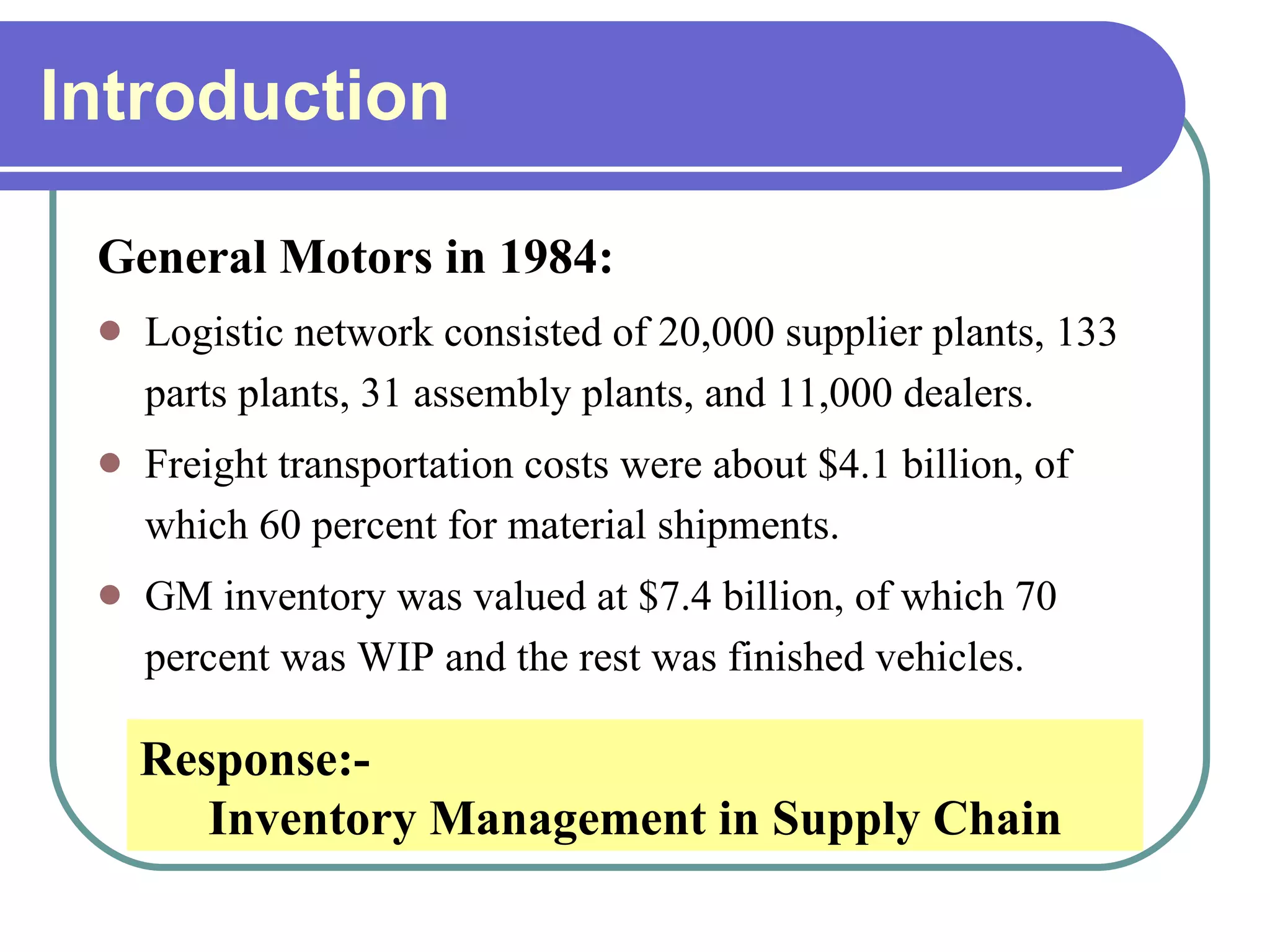
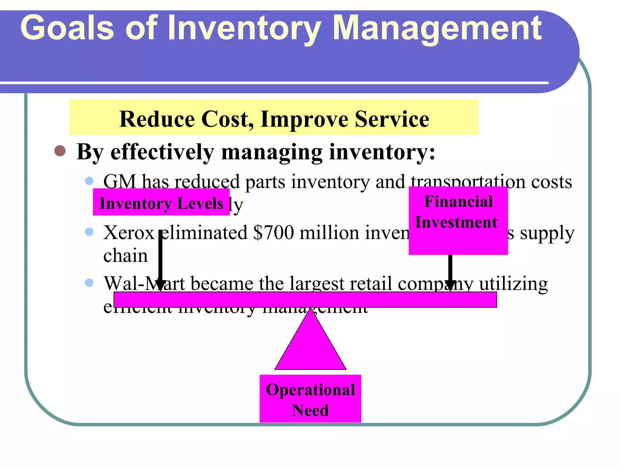
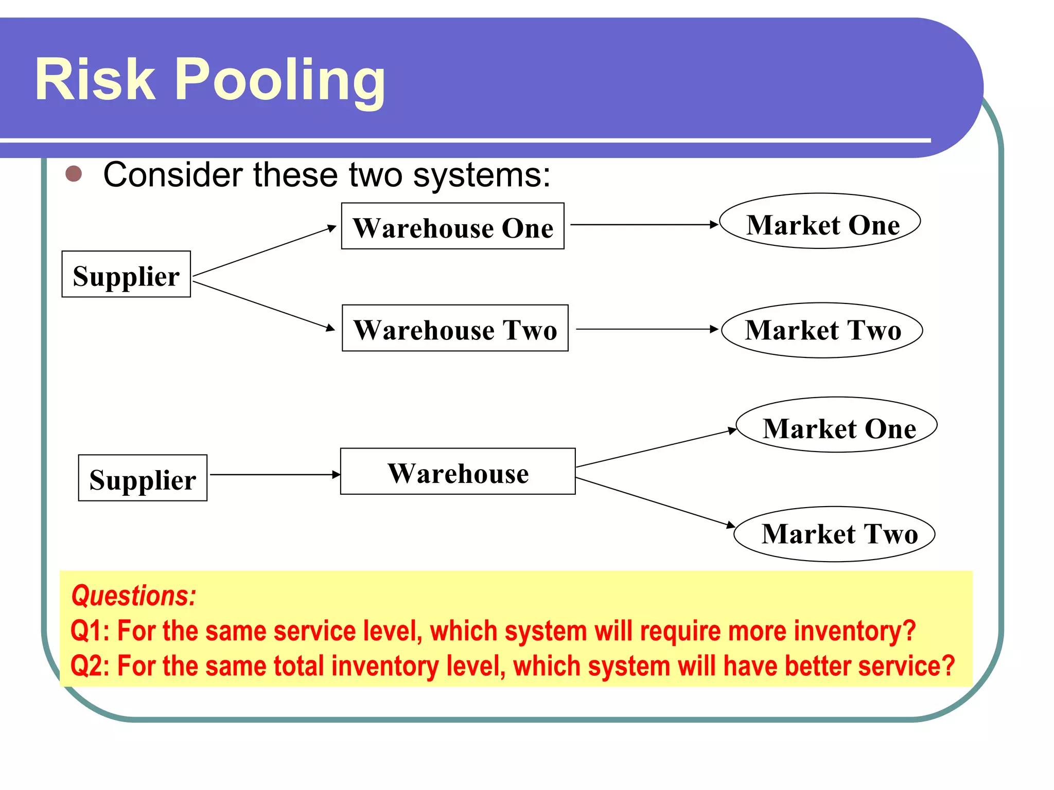
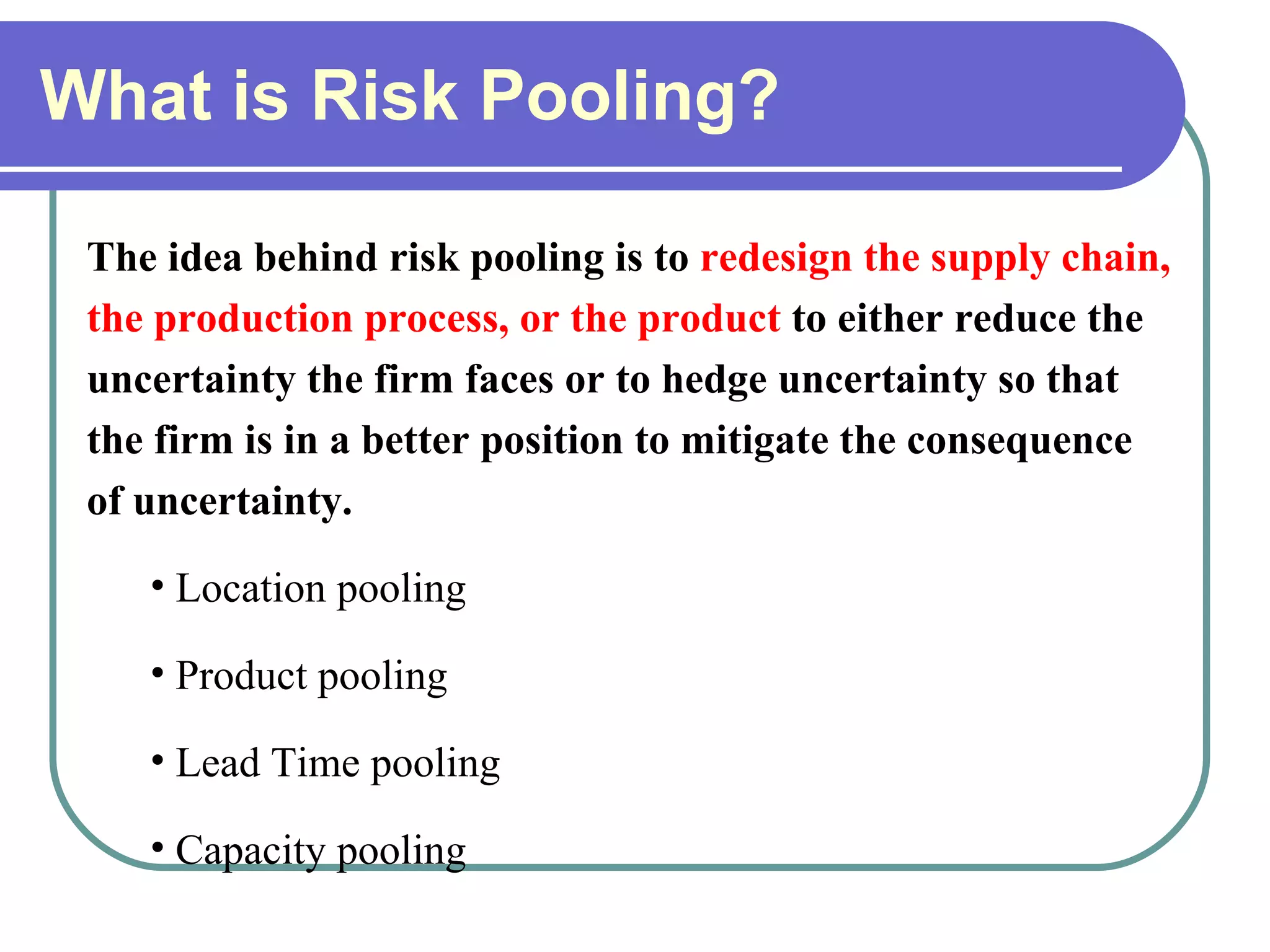
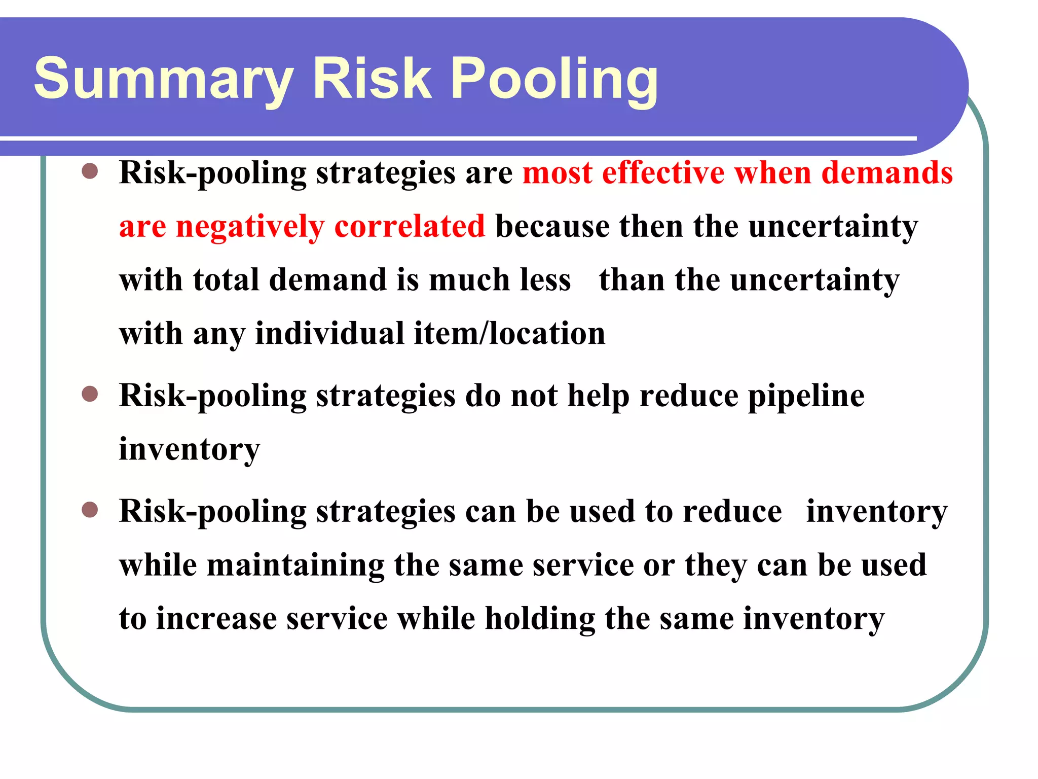
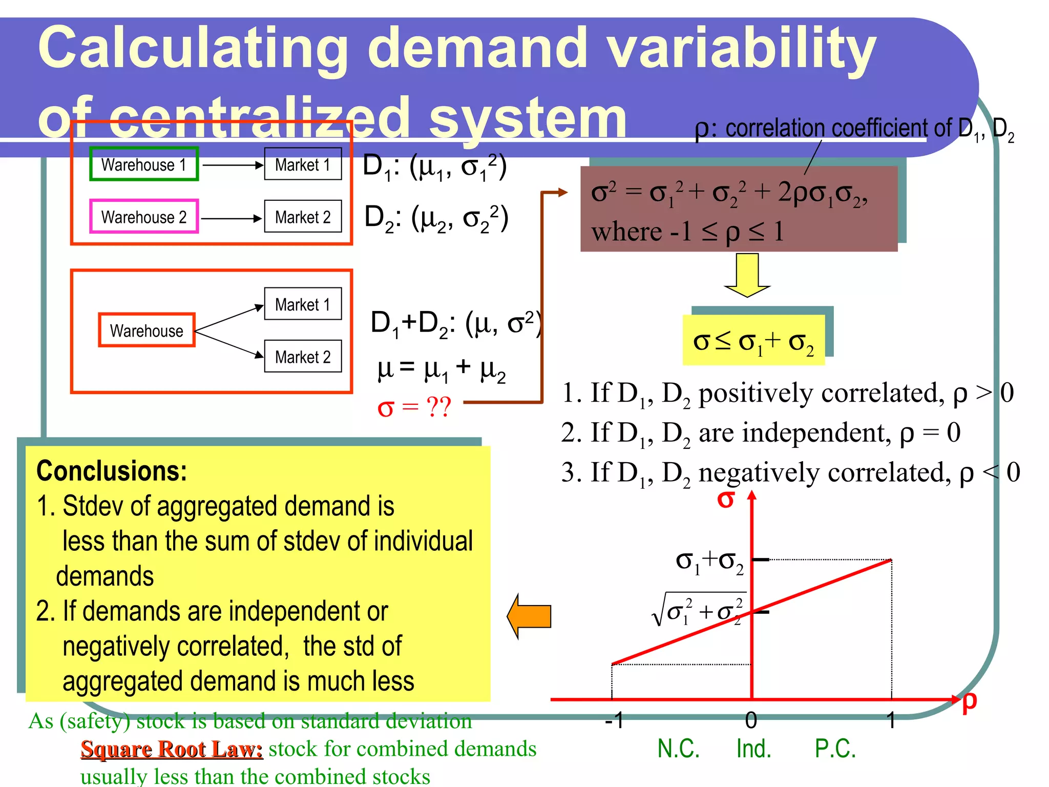
Inventory management and risk pooling are important concepts in supply chain management. General Motors in 1984 had a large logistic network with high inventory levels and transportation costs. Effective inventory management and risk pooling strategies can help companies reduce costs and improve customer service by reducing inventory levels while maintaining the same level of service or improving service with the same inventory. These strategies work best when demands across different locations are negatively correlated as it reduces overall demand variability.

1. Inventory Management & Risk Pooling

2. Introduction General Motors in 1984: Logistic network consisted of 20,000 supplier plants, 133 parts plants, 31 assembly plants, and 11,000 dealers. Freight transportation costs were about $4.1 billion, of which 60 percent for material shipments. GM inventory was valued at $7.4 billion, of which 70 percent was WIP and the rest was finished vehicles. Response:- Inventory Management in Supply Chain

3. Goals of Inventory Management By effectively managing inventory: GM has reduced parts inventory and transportation costs by 26% annually Xerox eliminated $700 million inventory from its supply chain Wal-Mart became the largest retail company utilizing efficient inventory management Reduce Cost, Improve Service Inventory Levels Financial Investment Operational Need

4. Inventory Where do we hold inventory? Suppliers and manufacturers warehouses and distribution centers retailers Types of Inventory : General classification WIP raw materials finished goods

5. Functions of Inventory To meet anticipated demand To smooth production requirements To decouple operations To protect against stock-outs To take advantage of order cycles To help hedge against price increases To take advantage of quantity discounts

6. Factors Affecting Inventory Policy Demand Characteristics: known in advance or random Lead Time Number of Different Products Stored in the Warehouse Economies of scale offered by suppliers & transport companies Length of Planning Horizon Service level desired

7. Economic Order Quantity Model Assuming demand certainty Trade-offs between setup costs and inventory holding costs, but ignores issues such as demand uncertainty and forecasting . 1000 2000 3000 4000 5000 6000 0 50 100 150 200 250 300 350 Ordering (Acquisition)Costs Holding or Carrying Costs Total Costs Economic Order Quantity

8. Single Period Model Without Initial Inventory

9. Case: Swimsuit Production A company designs, produces, and sells summer fashion items such as swinsuits. The company has to commit itself six months before summer to specific production quantities for all its products predicting demand for each product. The trade-offs are clear: overestimating customer demand will result in unsold inventory while underestimating customer demand will lead to inventory stockouts and loss of potential customers.

10. Demand forecast forecast averages about 13,000 The marketing department uses historical data from the last five years, current economic conditions, and other factors to construct a probabilistic forecast of the demand.

11. Swimsuit Costs Production cost per unit (C): $80 Selling price per unit (S): $125 Salvage value per unit (V): $20 Fixed production cost (F): $100,000 Q is production quantity, D: demand Profit = Revenue - Variable Cost - Fixed Cost + Salvage

12. Swimsuit Two Scenarios Scenario One: Suppose you make 12,000 jackets and demand ends up being 13,000 jackets. Profit = 125(12,000) - 80(12,000) - 100,000 = $440,000 Scenario Two: Suppose you make 12,000 jackets and demand ends up being 11,000 jackets. Profit = 125(11,000) - 80(12,000) - 100,000 + 20(1000) = $ 335,000

13. Swimsuit Best Questions ? Find order quantity that maximizes weighted average profit? Will this quantity be less than, equal to, or greater than average demand?

14. How much to Make? Marginal cost Vs. marginal profit if extra jacket sold, profit is 125-80 = 45 if not sold, cost is 80-20 = 60 So we will make less than average

15. Swimsuit Expected Profit

16. Swimsuit : Important Observations Tradeoff between ordering enough to meet demand and ordering too much Several quantities have the same average profit Average profit does not tell the whole story 9000 and 16000 units lead to about the same average profit, so which do we prefer?

17. Swimsuit Expected Profit

18. Case: Swimsuit Production But Need to understand risk associated with certain decisions. A frequency histogram provides information about potential profit for the two given production quantities, 9,000 units and 16,000 units. The possible risk and possible reward increases as we increase the production size.

19. Probability of Outcomes

20. Key Points from this Case The optimal order quantity is not necessarily equal to average forecast demand The optimal quantity depends on the relationship between marginal profit and marginal cost As order quantity increases, average profit first increases and then decreases As production quantity increases, risk increases. In other words, the probability of large gains and of large losses increases

21. Single Period Model With Initial Inventory

22. Initial Inventory Suppose that one of the jacket designs is a model produced last year. Some inventory is left from last year Assume the same demand pattern as before If only old inventory is sold, no setup cost Question: If there are 7000 units remaining, what should the company do? What should they do if there are 10,000 remaining?

23. Initial Inventory and Profit The case motivates a powerful ( s , S ) inventory policy (or a min max policy): s is the reorder point and S is the order-up-to-level

24. Multi-Order Opportunities under Uncertainties

25. Inventory Policies Continuous review policy in which inventory is reviewed every day and a decision is made about whether and how much to order. Periodic review policy in which the inventory level is reviewed at regular intervals and an appropriate quantity is ordered after each review.

26. Variable Demand with a Fixed ROP Reorder point, R Q LT Time LT Inventory level 0 Result of uncertainty

27. Reorder Point with a Safety Stock The amount of safety stock needed is based on the degree of uncertainty in the lead time demand and desired customer service level Reorder point, R Q LT Time LT Inventory level 0 Safety Stock

28. Determinants of the Reorder Point The rate of demand The lead time Demand and/or lead time variability Stockout risk (safety stock)

29. Continuous Review Policy AVG = Average daily demand faced STD = Standard deviation of daily demand faced L = Replenishment lead time h = Cost of holding one unit of the product per unit time α = service level (the probability of stocking out is 1 – α ) p =shortage cost

30. Continuous Review Policy The inventory position at any point in time is the actual inventory at the warehouse plus items ordered by the distributor that have not yet arrived minus items that are backordered . The reorder level, R consists of two components: the average inventory during lead time , which is the product of average daily demand and the lead time; and the safety stock , which is the amount of inventory that the distributor needs to keep at the warehouse and in the pipeline to protect against deviations from average demand during lead time.

31. Continuous Review Policy –Variable demand & fixed lead time Average demand during lead time is exactly Safety stock is where z is a constant, referred to as the safety factor . This constant is associated with the service level. The reorder level is Economic lot size is

32. Continuous Review Policy –Variable demand & fixed lead time The expected level of inventory before receiving the order is (lowest level i.e. Safety Stock) The expected level of inventory immediately after receiving the order is (highest level) The average inventory level is the average of these two values

33. In many situation, the lead time to the warehouse must be assumed to be normally distributed with average lead time denoted by AVGL and standard deviation denoted by STDL . In this case, the reorder point is calculated as where AVG x AVGL represents average demand during lead time, & is the standard deviation of demand during lead time. The amount of safety stock that has to be kept is equal to Continuous Review Policy –Variable demand & lead time

34. Periodic Review Policy Inventory level is reviewed periodically at regular intervals and an appropriate quantity so as to arrive at base stock level is ordered after each review . Since inventory levels are reviewed at a periodic interval, the fixed cost of placing an order is a sunk cost and hence can be ignored. This level of the inventory position should be enough to protect the warehouse against shortages until the next order arrives, that is to cover demand during a period of r + L days , with r being the length of review period and L being the lead time.

35. Periodic Review Policy Thus, the base-stock level should include two components: average demand during an interval of r + L days, which is equal to and the safety stock, which is calculated as where z is a safety factor.

36. Periodic Review Policy Maximum inventory level is achieved immediately after receiving an order, while the minimum level of inventory is achieved just before receiving an order. It is easy to see that the expected level of inventory after receiving an order is while the expected level of inventory before an order arrives is just the safety stock Hence, the average inventory level is the average of these two values

37. RISK POOLING

38. Risk Pooling Consider these two systems: Questions: Q1: For the same service level, which system will require more inventory? Q2: For the same total inventory level, which system will have better service? Market Two Supplier Warehouse One Warehouse Two Market One Market Two Supplier Warehouse Market One

39. What is Risk Pooling? The idea behind risk pooling is to redesign the supply chain, the production process, or the product to either reduce the uncertainty the firm faces or to hedge uncertainty so that the firm is in a better position to mitigate the consequence of uncertainty. Location pooling Product pooling Lead Time pooling Capacity pooling

40. Lead Time Pooling Supplier 8-week lead time

41. Lead Time Pooling Supplier 8-week lead time Retail DC 1-week lead time

42. Capacity Pooling 3 Links – no flexibility

43. Capacity Pooling 9 Links – Total Flexibility

44. Advantages / Disadvantages large costs to have flexibility accommodate demand uncertainty Capacity Pooling reduce inventory investment additional transportation costs keep inventory closer to customer extra costs of operating distribution center decrease lead time Lead Time Pooling better performance in terms of matching supply and demand potentially degrades product functionality reduction in demand variability Product Pooling reduce expected inventory investment needed to achieve a target service level creates distance between inventory and customers reduce demand variability Location Pooling Disadvantages Advantages

45. Summary Risk Pooling Risk-pooling strategies are most effective when demands are negatively correlated because then the uncertainty with total demand is much less than the uncertainty with any individual item/location Risk-pooling strategies do not help reduce pipeline inventory Risk-pooling strategies can be used to reduce inventory while maintaining the same service or they can be used to increase service while holding the same inventory

46. Example Decentralized system: total SS = 47.88 total avg. invent. = 179 Safety Stock SS = z · STD · Reorder Point R = AVG · L + SS Order Quantity Q = sqrt(2* C 0 *AVG/h ) Order-up-to-level R + Q Average Inventory  SS + Q/2 Service Level:97% k=1.88 Lead Time= 1 week Q/2+SS AVG STD SS R Q Order- up-to Level Average Inventory Warehouse 1 39.3 13.2 25.08 65 132 197 91 Warehouse 2 38.6 12.0 22.8 62 131 193 88 Centralized Warehouse 77.9 20.7 39.35 118 186 304 132

47. Risk Pooling – Effect of Correlation The benefits of risk pooling depend on the behavior of demand from one market relative to the demand from another market .

48. Warehouse Market 1 Market 2 D 1 +D 2 : (  ,  2 ) Calculating demand variability of centralized system Conclusions: 1. Stdev of aggregated demand is less than the sum of stdev of individual demands 2. If demands are independent or negatively correlated, the std of aggregated demand is much less 1. If D 1 , D 2 positively correlated,  > 0 2. If D 1 , D 2 are independent,  = 0 3. If D 1 , D 2 negatively correlated,  < 0  =  1 +  2  = ?? As (safety) stock is based on standard deviation Square Root Law: stock for combined demands usually less than the combined stocks Warehouse 1 Warehouse 2 Market 1 Market 2 D 1 : (  1 ,  1 2 ) D 2 : (  2 ,  2 2 )  2 =  1 2 +  2 2 + 2  1  2 , where -1    1  : correlation coefficient of D 1 , D 2    1 +  2    1 +  2 1 0 -1 P.C. N.C. Ind.

49. Risk Pooling – Effect of Coefficient of Variation The higher the C.V . of demand observed in one market, the greater the benefit from risk pooling COV= Standard deviation/Avg. demand

50. Decentralized Centralized Inbound transportation cost (from factories to warehouses) Facility/Labor cost Outbound transportation cost (from warehouses to retailers) Safety Stock Responsiveness to customers (lead time) Centralized vs. Decentralized Overhead Costs Service Level

51. Case Study # below stage = processing time # in white box = CST In this solution, inventory is held of finished product and its raw materials (Adapted from Simchi-Levi, Chen, and Bramel, The Logic of Logistics , Springer, 2004) PART 1 DALLAS ($260) 15 7 8 PART 2 CHARLESTON ($7) 14 PART 4 BALTIMORE ($220) 5 PART 3 AUSTIN ($2) 14 6 8 5 PART 5 CHICAGO ($155) 45 PART 7 CHARLESTON ($30) 14 PART 6 CHARLESTON ($2) 32 8 0 14 55 14 45 14 32

52. A Pure Pull System Produce to order Long CST to customer No inventory held in system PART 1 DALLAS ($260) 15 7 8 PART 2 CHARLESTON ($7) 14 PART 4 BALTIMORE ($220) 5 PART 3 AUSTIN ($2) 14 6 8 5 PART 5 CHICAGO ($155) 45 PART 7 CHARLESTON ($30) 14 PART 6 CHARLESTON ($2) 32 8 77 14 55 14 45 14 32

53. A Pure Push System Produce to forecast Zero CST to customer Hold lots of finished goods inventory PART 1 DALLAS ($260) 15 7 8 PART 2 CHARLESTON ($7) 14 PART 4 BALTIMORE ($220) 5 PART 3 AUSTIN ($2) 14 6 8 5 PART 5 CHICAGO ($155) 45 PART 7 CHARLESTON ($30) 14 PART 6 CHARLESTON ($2) 32 8 0 14 55 14 45 14 32

54. A Hybrid Push-Pull System Part of system operated produce-to-stock, part produce-to-order Moderate lead time to customer PART 1 DALLAS ($260) 15 7 8 PART 2 CHARLESTON ($7) 14 PART 4 BALTIMORE ($220) 5 PART 3 AUSTIN ($2) 14 6 8 5 PART 5 CHICAGO ($155) 45 PART 7 CHARLESTON ($30) 14 PART 6 CHARLESTON ($2) 32 8 30 7 8 9 45 14 32 push/pull boundary

55. CST vs. Inventory Cost Push System Pull System Push-Pull System

56. Echelon Inventory System Supplier Warehouse Retailers Warehouse echelon inventory Warehouse echelon lead time

57. Managing Inventory in the Supply Chain How should the reorder point associated with the warehouse echelon inventory position be calculated? The reorder point is where L e = echelon lead time, defined as the lead time between the retailers and the warehouse plus the lead time between the warehouse and its supplier AVG = average demand across all retailers (i.e., the average of the aggregate demand) STD = standard deviation of (aggregate) demand across all retailers

58. Forecasting Recall the three rules Nevertheless, forecast is critical General Overview: Judgment methods Market research methods Time Series methods Causal methods

59. THANKYOU