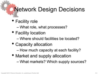
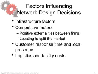
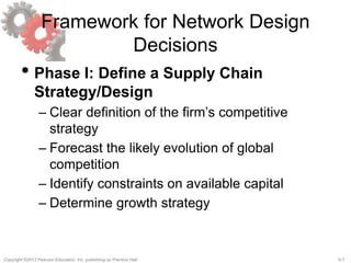
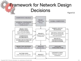
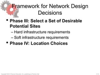
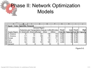
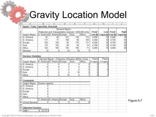
This document discusses network design in supply chains. It begins by outlining the key network design decisions, including facility role, location, capacity allocation, and market/supply allocation. It then discusses factors that influence these decisions, such as strategic, technological, economic, political, infrastructure, and competitive factors. The document presents a framework for network design decisions involving defining strategy, regional configuration, site selection, and location choices. It concludes by describing models that can be used for facility location and capacity allocation decisions, including a capacitated plant location model and gravity location model.

1. PowerPoint presentation to accompany
Chopra and Meindl Supply Chain Management, 5e
1-1
Copyright ©2013 Pearson Education, Inc. publishing as Prentice Hall.Copyright ©2013 Pearson Education, Inc. publishing as Prentice Hall.Copyright ©2013 Pearson Education, Inc. publishing as Prentice Hall.
1-1
Copyright ©2013 Pearson Education, Inc. publishing as Prentice Hall.
1-1
Copyright ©2013 Pearson Education, Inc. publishing as Prentice Hall.
5-1
Copyright ©2013 Pearson Education, Inc. publishing as Prentice Hall.
Network Design in
the Supply Chain
5

2. 5-2Copyright ©2013 Pearson Education, Inc. publishing as Prentice Hall.
Learning Objectives
1. Understand the role of network design in a
supply chain.
2. Identify factors influencing supply chain
network design decisions.
3. Develop a framework for making network
design decisions.
4. Use optimization for facility location and
capacity allocation decisions.

3. 5-3Copyright ©2013 Pearson Education, Inc. publishing as Prentice Hall.
Network Design Decisions
• Facility role
– What role, what processes?
• Facility location
– Where should facilities be located?
• Capacity allocation
– How much capacity at each facility?
• Market and supply allocation
– What markets? Which supply sources?

4. 5-4Copyright ©2013 Pearson Education, Inc. publishing as Prentice Hall.
Factors Influencing
Network Design Decisions
• Strategic factors
• Technological factors
• Macroeconomic factors
– Tariffs and tax incentives
– Exchange-rate and demand risk
– Freight and fuel costs
• Political

5. 5-5Copyright ©2013 Pearson Education, Inc. publishing as Prentice Hall.
Factors Influencing
Network Design Decisions
• Infrastructure factors
• Competitive factors
– Positive externalities between firms
– Locating to split the market
• Customer response time and local
presence
• Logistics and facility costs

6. 5-6Copyright ©2013 Pearson Education, Inc. publishing as Prentice Hall.
Competitive Factors
– Positive externalities between firms
• Collocation benefits all
– Locating to split the market
• Locate to capture largest market share
d1
= a +
1– b – a
2
and d2
=
1+ b – a
2
Figure 5-1

7. 5-7Copyright ©2013 Pearson Education, Inc. publishing as Prentice Hall.
Framework for Network Design
Decisions
• Phase I: Define a Supply Chain
Strategy/Design
– Clear definition of the firm’s competitive
strategy
– Forecast the likely evolution of global
competition
– Identify constraints on available capital
– Determine growth strategy

8. 5-8Copyright ©2013 Pearson Education, Inc. publishing as Prentice Hall.
Framework for Network Design
Decisions Figure 5-2

9. 5-9Copyright ©2013 Pearson Education, Inc. publishing as Prentice Hall.
Framework for Network Design
Decisions
• Phase II: Define the Regional Facility
Configuration
– Forecast of the demand by country or region
– Economies of scale or scope
– Identify demand risk, exchange-rate risk,
political risk, tariffs, requirements for local
production, tax incentives, and export or
import restrictions
– Identify competitors

10. 5-10Copyright ©2013 Pearson Education, Inc. publishing as Prentice Hall.
Framework for Network Design
Decisions
• Phase III: Select a Set of Desirable
Potential Sites
– Hard infrastructure requirements
– Soft infrastructure requirements
• Phase IV: Location Choices

11. 5-11Copyright ©2013 Pearson Education, Inc. publishing as Prentice Hall.
Models for Facility Location and
Capacity Allocation
• Maximize the overall profitability of the
supply chain network while providing
customers with the appropriate
responsiveness
• Many trade-offs during network design
• Network design models used to decide on
locations and capacities and to assign
current demand to facilities

12. 5-12Copyright ©2013 Pearson Education, Inc. publishing as Prentice Hall.
Models for Facility Location and
Capacity Allocation
• Important information
– Location of supply sources and markets
– Location of potential facility sites
– Demand forecast by market
– Facility, labor, and material costs by site
– Transportation costs between each pair of sites
– Inventory costs by site and as a function of quantity
– Sale price of product in different regions
– Taxes and tariffs
– Desired response time and other service factors

13. 5-13Copyright ©2013 Pearson Education, Inc. publishing as Prentice Hall.
Phase II: Network Optimization
Models
Figure 5-3

14. 5-14Copyright ©2013 Pearson Education, Inc. publishing as Prentice Hall.
Capacitated Plant Location Model
= number of potential plant locations/capacityn
m
Dj
Ki
fi
cij
= number of markets or demand points
= annual demand from market j
= potential capacity of plant i
= annualized fixed cost of keeping plant i open
= cost of producing and shipping one unit from plant i to market j (cost
includes production, inventory, transportation, and tariffs)
yi
xij = quantity shipped from plant i
to market j
= 1 if plant i is open, 0 otherwise
Min fi
yi
+
i=1
n
å cij
xij
j=1
m
å
i=1
n
å
subject to
xij
= Dj
for j =1,...,m
i=1
n
å
xij
j=1
m
å = Ki
yi
for i =1,...,n
yi
Î 0,1{ } for i =1,...,n,x ij
³ 0

15. 5-15Copyright ©2013 Pearson Education, Inc. publishing as Prentice Hall.
Capacitated Plant Location Model
Figure 5-4

16. 5-16Copyright ©2013 Pearson Education, Inc. publishing as Prentice Hall.
Capacitated Plant Location Model
Figure 5-5

17. 5-17Copyright ©2013 Pearson Education, Inc. publishing as Prentice Hall.
Capacitated Plant Location Model
Figure 5-5

18. 5-18Copyright ©2013 Pearson Education, Inc. publishing as Prentice Hall.
Phase III: Gravity Location Models
Figure 5-6

19. 5-19Copyright ©2013 Pearson Education, Inc. publishing as Prentice Hall.
Gravity Location Model
xn, yn: coordinate location of either a market or supply source n
Fn: cost of shipping one unit for one mile between the facility
and either market or supply source n
Dn: quantity to be shipped between facility and market or
supply source n
(x, y) is the location selected for the facility, the distance dn between
the facility at location (x, y) and the supply source or market n is given
by
dn
= x – xn( )
2
+ y – yn( )
2

20. 5-20Copyright ©2013 Pearson Education, Inc. publishing as Prentice Hall.
Gravity Location Model
Figure 5-7

21. 5-21Copyright ©2013 Pearson Education, Inc. publishing as Prentice Hall.
Gravity Location Model
Table 5-1
Sources/Market
s
Transportation Cost
$/Ton Mile (Fn)
Quantity in Tons
(Dn)
Coordinates
xn yn
Supply sources
Buffalo 0.90 500 700 1,200
Memphis 0.95 300 250 600
St. Louis 0.85 700 225 825
Markets
Atlanta 1.50 225 600 500
Boston 1.50 150 1,050 1,200
Jacksonville 1.50 250 800 300
Philadelphia 1.50 175 925 975
New York 1.50 300 1,000 1,080
Total transportation cost TC = dn
Dn
Fn
n=1
k
å

22. 5-22Copyright ©2013 Pearson Education, Inc. publishing as Prentice Hall.
Gravity Location Model
Figure 5-8

23. 5-23Copyright ©2013 Pearson Education, Inc. publishing as Prentice Hall.
Gravity Location Model
Figure 5-8

24. 5-24Copyright ©2013 Pearson Education, Inc. publishing as Prentice Hall.
Gravity Location Model
1. For each supply source or market n, evaluate dn
2. Obtain a new location (x’, y’) for the facility, where
¢x =
Dn
Fn
xn
dnn=1
k
å
Dn
Fn
dnn=1
k
å
and ¢y =
Dn
Fn
yn
dnn=1
k
å
Dn
Fn
dnn=1
k
å
3. If the new location (x’ , y’ ) is almost the same as
(x, y) stop. Otherwise, set (x, y) = (x’ , y’ ) and go to
step 1

25. 5-25Copyright ©2013 Pearson Education, Inc. publishing as Prentice Hall.
Phase IV: Network Optimization
Models
Supply
City
Demand City
Production and Transportation Cost
per Thousand Units (Thousand $)
Monthly
Capacity
(Thousand
Units) K
Monthly
Fixed Cost
(Thousand
$) fAtlanta Boston
Chicag
o Denver Omaha Portland
Baltimore 1,675 400 985 1,630 1,160 2,800 18 7,650
Cheyenne 1,460 1,940 970 100 495 1,200 24 3,500
Salt Lake
City
1,925 2,400 1,450 500 950 800 27 5,000
Memphis 380 1,355 543 1,045 665 2,321 22 4,100
Wichita 922 1,646 700 508 311 1,797 31 2,200
Monthly
demand
(thousand
units) Dj
10 8 14 6 7 11
Table 5-2

26. 5-26Copyright ©2013 Pearson Education, Inc. publishing as Prentice Hall.
Network Optimization Models
• Allocating demand to production facilities
= number of factory locationsn
m
Dj
Ki
cij
= number of markets or demand points
= annual demand from market j
= capacity of factory i
= cost of producing and shipping one unit from factory i to market j
xij = quantity shipped from
factory i to market j
Min cij
xij
j=1
m
å
i=1
n
å
subject to
xij
= Dj
for j =1,...,m
i=1
n
å
xij
j=1
m
å = Ki
for i =1,...,n

27. 5-27Copyright ©2013 Pearson Education, Inc. publishing as Prentice Hall.
Network Optimization Models
• Optimal demand allocation
Atlanta Boston Chicago Denver Omaha Portland
TelecomOne Baltimore 0 8 2
Memphis 10 0 12
Wichita 0 0 0
HighOptic Salt Lake 0 0 11
Cheyenne 6 7 0
Table 5-3

28. 5-28Copyright ©2013 Pearson Education, Inc. publishing as Prentice Hall.
Capacitated Plant Location Model
• Merge the companies
• Solve using location-specific costs
yi = 1 if factory i is open, 0 otherwise
xij = quantity shipped from factory i to market j
Min fi
yi
+
i=1
n
å cij
xij
j=1
m
å
i=1
n
å

29. 5-29Copyright ©2013 Pearson Education, Inc. publishing as Prentice Hall.
Capacitated Plant Location Model
Figure 5-9

30. 5-30Copyright ©2013 Pearson Education, Inc. publishing as Prentice Hall.
Capacitated Plant Location Model
Figure 5-10

31. 5-31Copyright ©2013 Pearson Education, Inc. publishing as Prentice Hall.
Capacitated Plant Location Model
Figure 5-10

32. 5-32Copyright ©2013 Pearson Education, Inc. publishing as Prentice Hall.
Capacitated Plant Location Model
Figure 5-11

33. 5-33Copyright ©2013 Pearson Education, Inc. publishing as Prentice Hall.
Capacitated Model With
Single Sourcing
• Market supplied by only one factory
• Modify decision variables
yi = 1 if factory i is open, 0 otherwise
xij = 1 if market j is supplied by factory i, 0 otherwise
Min fi
yi
+ Dj
cij
xij
j=1
m
å
i=1
n
å
i=1
n
å
subject to
xij
=1 for j =1,...,m
i=1
n
å
Di
xij
£ Ki
yi
j=1
m
å for i =1,...,n
xij
, yi
Î 0,1{ }

34. 5-34Copyright ©2013 Pearson Education, Inc. publishing as Prentice Hall.
Capacitated Model With
Single Sourcing
Figure 5-12

35. 5-35Copyright ©2013 Pearson Education, Inc. publishing as Prentice Hall.
Capacitated Model With
Single Sourcing
• Optimal network configuration with single
sourcing
Open/
Closed Atlanta Boston Chicago Denver Omaha Portland
Baltimore Closed 0 0 0 0 0 0
Cheyenne Closed 0 0 0 0 0 0
Salt Lake Open 0 0 0 6 0 11
Memphis Open 10 8 0 0 0 0
Wichita Open 0 0 14 0 7 0
Table 5-4

36. 5-36Copyright ©2013 Pearson Education, Inc. publishing as Prentice Hall.
Locating Plants and Warehouses
Simultaneously
Figure 5-13

37. 5-37Copyright ©2013 Pearson Education, Inc. publishing as Prentice Hall.
Locating Plants and Warehouses
Simultaneously
• Model inputs
m = number of markets or demand points
n = number of potential factory locations
l = number of suppliers
t = number of potential warehouse locations
Dj = annual demand from customer j
Ki = potential capacity of factory at site i
Sh = supply capacity at supplier h
We = potential warehouse capacity at site e
Fi = fixed cost of locating a plant at site i
fe = fixed cost of locating a warehouse at site e
chi = cost of shipping one unit from supply source h to factory i
cie = cost of producing and shipping one unit from factory i to warehouse e
cej = cost of shipping one unit from warehouse e to customer j

38. 5-38Copyright ©2013 Pearson Education, Inc. publishing as Prentice Hall.
Locating Plants and Warehouses
Simultaneously
• Goal is to identify plant and warehouse locations
and quantities shipped that minimize the total
fixed and variable costs
Yi = 1 if factory is located at site i, 0 otherwise
Ye = 1 if warehouse is located at site e, 0 otherwise
xej = quantity shipped from warehouse e to market j
xie = quantity shipped from factory at site i to warehouse e
xhi = quantity shipped from supplier h to factory at site i
Min Fi
yi
+ fe
ye
+ chi
xie
i=1
n
å + cej
xej
j=1
m
å
e=1
t
å
h=1
l
å
e=1
t
å
i=1
n
å

39. 5-39Copyright ©2013 Pearson Education, Inc. publishing as Prentice Hall.
Locating Plants and Warehouses
Simultaneously
subject to
xhi
£ Sh
for h =1,...,l
i=1
n
å
xhi
– xie
e=1
t
å ³ 0 for i =1,...,n
h=1
l
å
xie
£ Ki
yi
for i =1,...,n
e=1
t
å
xie
– xej
j=1
m
å ³ 0 for e =1,...,t
i=1
n
å
xej
£We
ye
for e =1,...,t
j=1
m
å
xej
= Dj
for j =1,...,m
e=1
t
å
yi
, ye
Î 0,1{ },xej
,xie
,xhi
³ 0

40. 5-40Copyright ©2013 Pearson Education, Inc. publishing as Prentice Hall.
Accounting for Taxes, Tariffs, and
Customer Requirements
• A supply chain network should maximize profits
after tariffs and taxes while meeting customer
service requirements
• Modified objective and constraint
Max rj
xij
– Fi
yi
– cij
xij
j=1
m
å
i=1
n
å
i=1
n
å
i=1
n
å
j=1
m
å
xij
£ Dj
for j =1,...,m
i=1
n
å

41. 5-41Copyright ©2013 Pearson Education, Inc. publishing as Prentice Hall.
Making Network Design Decisions
In Practice
• Do not underestimate the life span of
facilities
• Do not gloss over the cultural
implications
• Do not ignore quality-of-life issues
• Focus on tariffs and tax incentives
when locating facilities

42. 5-42Copyright ©2013 Pearson Education, Inc. publishing as Prentice Hall.
Summary of Learning Objectives
1. Understand the role of network design
in a supply chain
2. Identify factors influencing supply
chain network design decisions
3. Develop a framework for making
network design decisions
4. Use optimization for facility location
and capacity allocation decisions

43. 5-43Copyright ©2013 Pearson Education, Inc. publishing as Prentice Hall.
All rights reserved. No part of this publication may be reproduced, stored in a retrieval
system, or transmitted, in any form or by any means, electronic, mechanical, photocopying,
recording, or otherwise, without the prior written permission of the publisher.
Printed in the United States of America.