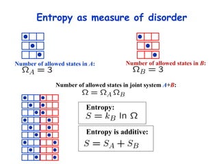
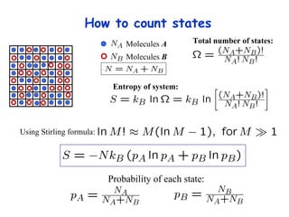
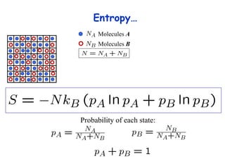
![Thermodynamics of open systems (reaction mixes) For one component (A): G A = G A °´ + n A RT .ln[ A ] And for 1 mole of A: where the units are free energy per mole (J mol -1 ). This quantity is also known as the chemical potential (µ A ) and we write: µ A = µ A °´ + RT .ln[ A ] Previously we had for the general case: dG = Vdp - SdT For open, multicomponent systems, we write: dG = Vdp - SdT + i µ i dn i](https://image.slidesharecdn.com/introductory-biological-thermodynamics-29750/85/Introductory-biological-thermodynamics-21-320.jpg)
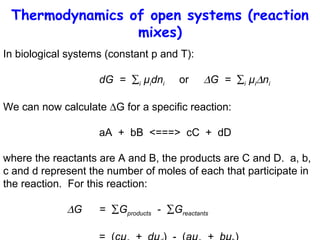
![Thermodynamics of open systems (reaction mixes) But µ A = µ A °´ + RT. ln[A] etc . so: G = [(cµ c °´ + dµ d °´) - (aµ a °´ + bµ b °´) + RT ln ( [C] c [D] d /[A] a [B] b ) which we express as: G = G°´ + RT ln ( [C] c [D] d /[A] a [B] b ) (Joules) To find the free energy change per mole , note that a, b, c and d will reflect the stoichiometry of the reaction (the numbers of each type of molecule involved in a single reaction). For example, a single reaction might involve the following numbers of molecules: 2A + 1B <----> 1C + 2D which is the same as: A + A + B <----> C + D + D](https://image.slidesharecdn.com/introductory-biological-thermodynamics-29750/85/Introductory-biological-thermodynamics-23-320.jpg)
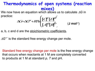
![Thermodynamic equilibrium We calculate G so that we can determine the spontaneous direction of a reaction (favourable or unfavourable). To do that we must determine: G°´ the concentration of each component the stoichiometry of the reaction. We need G < 0 for a favourable forward reaction. We can drive the reaction forward either by: increasing [A] and/or [B] decreasing [C] and/or [D] Living cells can (sometimes) control reactant/product concentrations to ensure that G < 0 for desired reactions.](https://image.slidesharecdn.com/introductory-biological-thermodynamics-29750/85/Introductory-biological-thermodynamics-25-320.jpg)
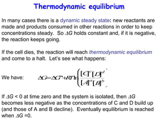
![Thermodynamic equilibrium Note: if G°´ < 0, then ([C][D]) eq > ([A][B]) eq (for a=b=c=d=1) if G°´ > 0, then ([C][D]) eq < ([A][B]) eq Thus, G°´ determines whether the reactants or products predominate at equilibrium. T Thermodynamic equilibrium is not a static state (conversion of A and B to C and D and back again keeps going but there is no net change in their concentrations).](https://image.slidesharecdn.com/introductory-biological-thermodynamics-29750/85/Introductory-biological-thermodynamics-28-320.jpg)

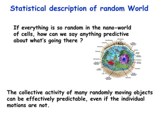
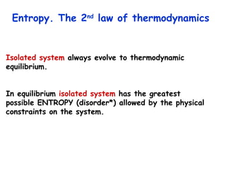
This lecture introduces concepts of thermodynamics and how they relate to living systems. It discusses how living systems maintain order far from equilibrium and uses energy and molecular interactions. Key concepts covered include entropy, Gibbs free energy, and how biological systems can direct spontaneous reactions through non-equilibrium conditions and concentration control. Thermodynamic equilibrium is defined and how the sign of change in Gibbs free energy determines reaction direction.


