Download as PDF, PPTX


![Binary variable: Bernoulli
Let us consider a single binary random variable x ∈ {0, 1}, e.g. flipping coin, not necessary
fair, hence the probability is conditioned by a parameter 0 ≤ µ ≤ 1:
p(x = 1|µ) = µ (7)
The probability distribution over x is known as the Bernoulli distribution:
Bern(x|µ) = µx
(1 − µ)1−x
(8)
E[x] = µ (9)
9](https://image.slidesharecdn.com/edl-intro-200530175739/75/Introduction-to-Evidential-Neural-Networks-9-2048.jpg)
![Binomial distribution
The distribution of m observations of x = 1 given the datasize N is given by the Binomial
distribution:
Bin(m|N, µ) =
N
m
µm
(1 − µ)N−m
(10)
with
E[m] ≡
N
m=0
mBin(m|N, µ) = Nµ (11)
and
var[m] ≡
N
m=0
(m − E[m])2
Bin(m|N, µ) = Nµ(1 − µ) (12)
10
Image from Bishop, C. M. Pattern Recognition and Machine Learning. (Springer-Verlag, 2006).](https://image.slidesharecdn.com/edl-intro-200530175739/75/Introduction-to-Evidential-Neural-Networks-10-2048.jpg)


![Binary variables: Beta distribution
Beta(µ|a, b) =
Γ(a + b)
Γ(a)Γ(b)
µa−1
(1 − µ)b−1
with
Γ(x) ≡
∞
0
ux−1
e−u
du
E[µ] =
a
a + b
var[µ] =
ab
(a + b)2(a + b + 1)
a and b are hyperparameters controlling the distribution of parameter µ.
16](https://image.slidesharecdn.com/edl-intro-200530175739/75/Introduction-to-Evidential-Neural-Networks-16-2048.jpg)


![Loss function
If we then consider Dir(mi | αi ) as the prior for a Multinomial p(yi | µi ), we can then compute the
expected squared error (aka Brier score)
E[ yi − mi
2
2
] =
K
k=1
E[y2
i,k − 2yi,k µi,k + µ2
i,k ] =
X
k=1
y2
i,k − 2yi,k E[µi,k ] + E[µ2
i,k ] =
=
K
k=1
y2
i,k − 2yi,k E[µi,k ] + E[µi,k ]2
+ var[µi,k ] =
=
K
k=1
(yi,k − E[µi,k ])2
+ var[µi,k ] =
=
K
k=1
yi,k −
αi,k
Si
2
+
αi,k (Si − αi,k )
S2
i (Si + 1)
=
=
K
k=1
(yi,k − µi,k )2
+
µi,k (1 − µi,k )2
Si + 1
The loss over a batch of training samples is the sum of the loss for each sample in the batch.
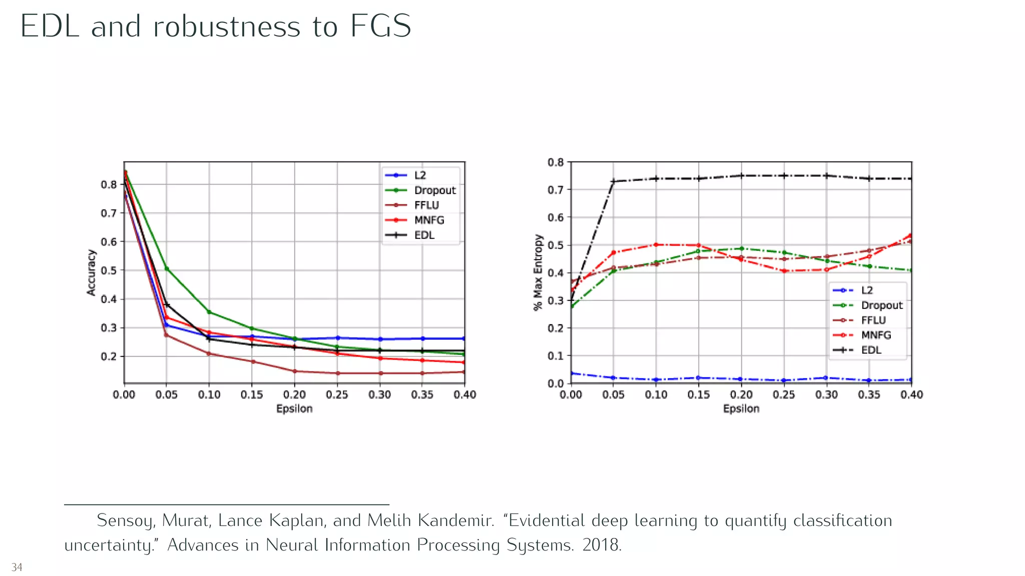
Sensoy, Murat, Lance Kaplan, and Melih Kandemir. “Evidential deep learning to quantify classification
uncertainty.” Advances in Neural Information Processing Systems. 2018.
30](https://image.slidesharecdn.com/edl-intro-200530175739/75/Introduction-to-Evidential-Neural-Networks-30-2048.jpg)
![Learning to say “I don’t know”
To avoid generating evidence for all the classes when the network cannot classify a given
sample (epistemic uncertainty), we introduce a term in the loss function that penalises the
divergence from the uniform distribution:
L =
N
i=1
E[ yi − µi
2
2
] + λt
N
i=1
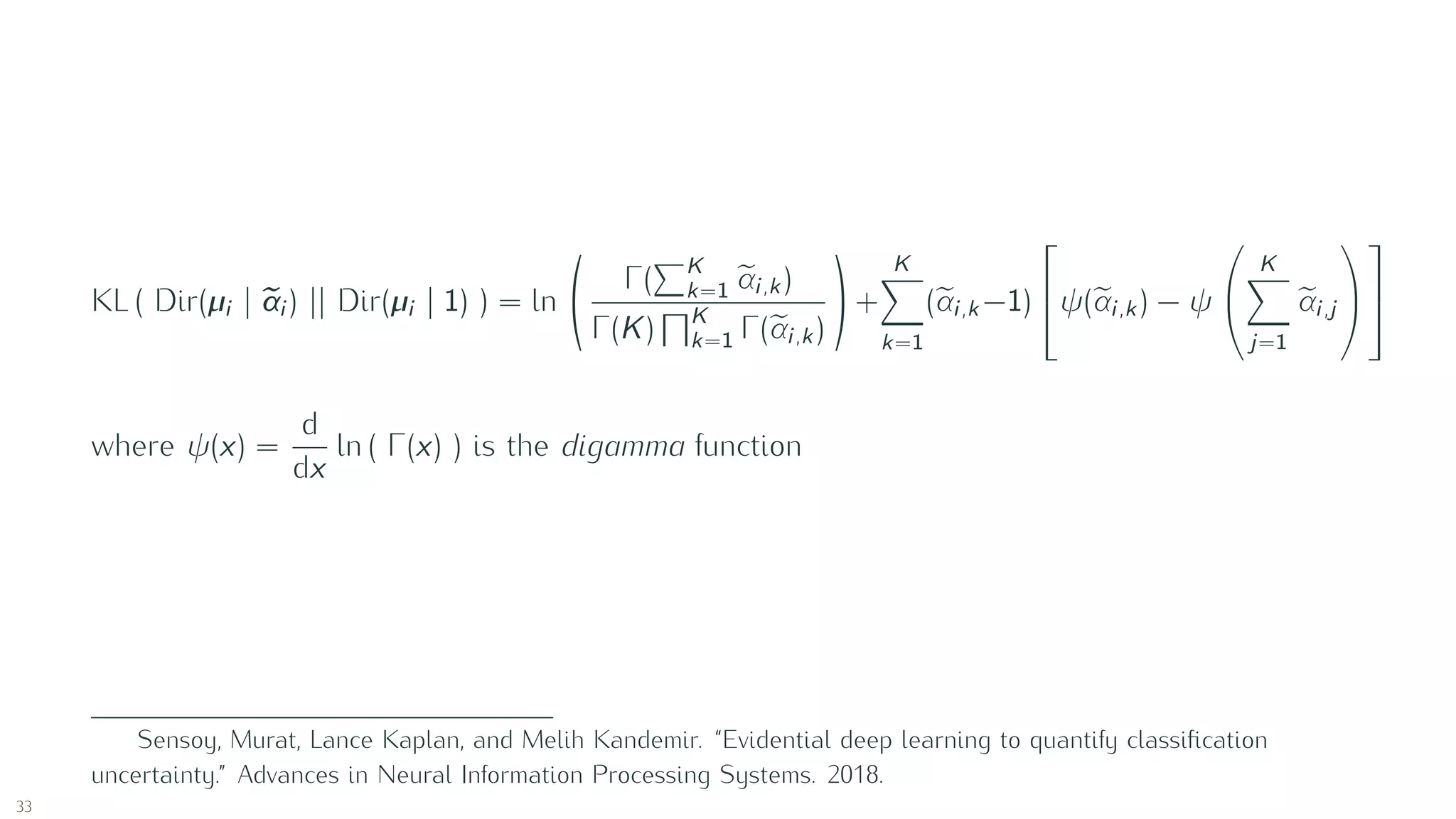
KL ( Dir(µi | αi ) || Dir(µi | 1) )
where:
• λt is another hyperparameter, and the suggestion is to use it parametric on the number of
training epochs, e.g. λt = min 1,
t
CONST
with t the number of current training epoch, so that
the effect of the KL divergence is gradually increased to avoid premature convergence to the
uniform distribution in the early epoch where the learning algorithm still needs to explore the
parameter space;
• αi = yi + (1 − yi ) · αi are the Dirichlet parameters the neural network in a forward pass has put
on the wrong classes, and the idea is to minimise them as much as possible.
Sensoy, Murat, Lance Kaplan, and Melih Kandemir. “Evidential deep learning to quantify classification
uncertainty.” Advances in Neural Information Processing Systems. 2018.
31](https://image.slidesharecdn.com/edl-intro-200530175739/75/Introduction-to-Evidential-Neural-Networks-31-2048.jpg)


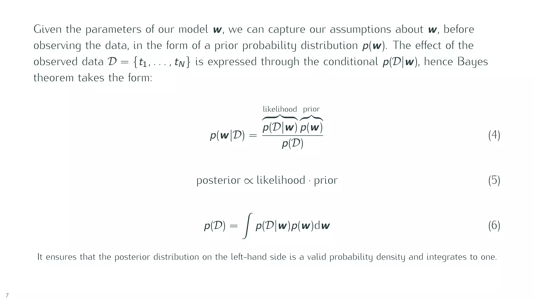
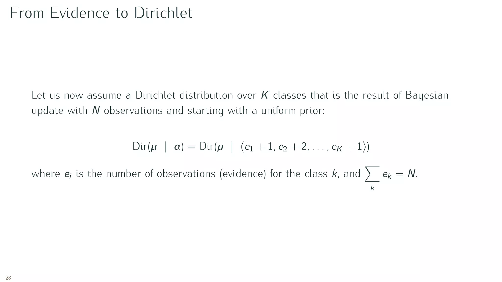
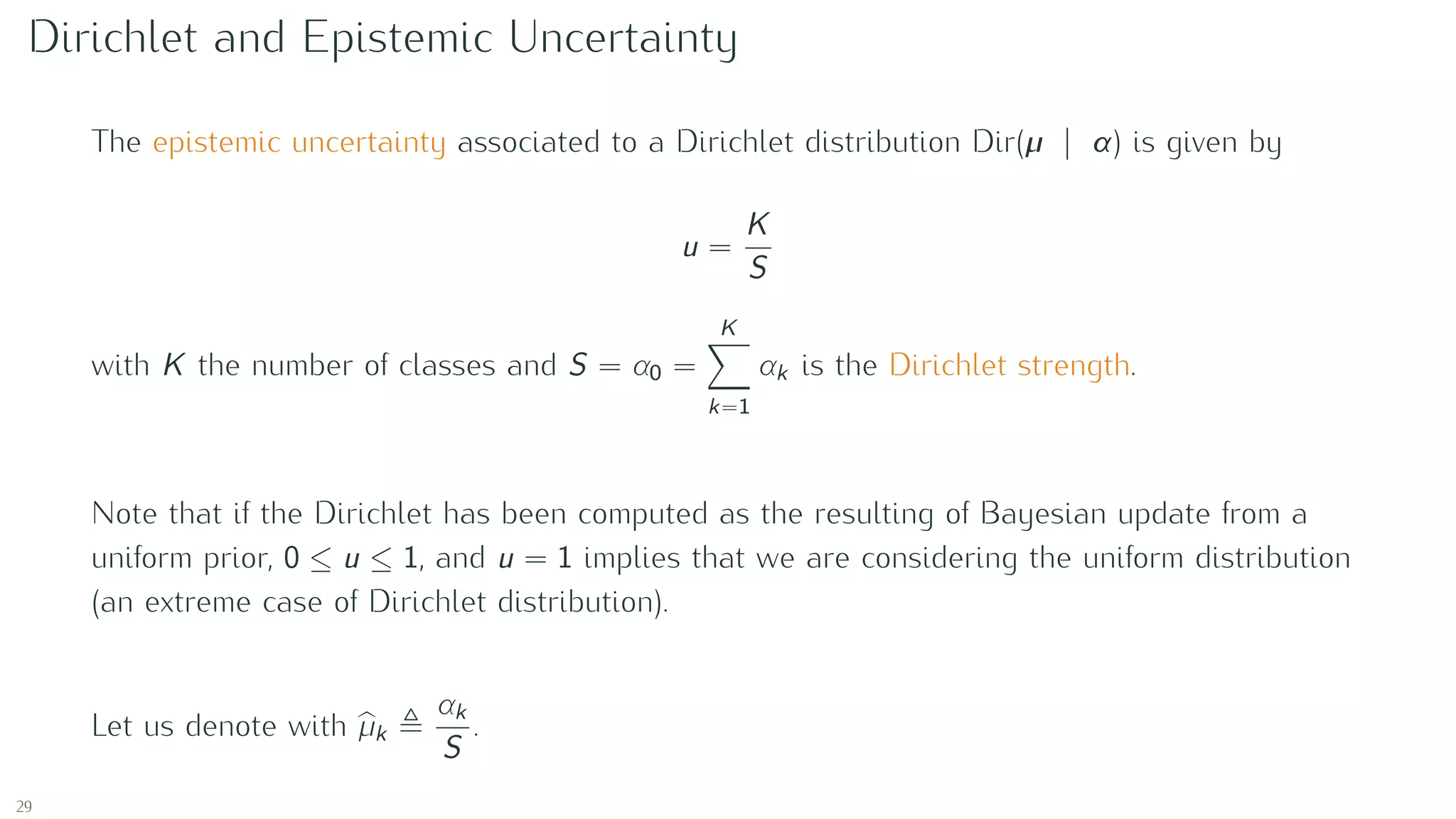
This document provides an introduction to Bayesian analysis and probabilistic modeling. It begins with an overview of Bayes' theorem and common probability distributions used in Bayesian modeling like the Bernoulli, binomial, beta, Dirichlet, and multinomial distributions. It then discusses how these distributions can be used in Bayesian modeling for problems like estimating probabilities based on observed data. Specifically, it explains how conjugate prior distributions allow the posterior distribution to be of the same family as the prior. The document concludes by discussing how neural networks can quantify classification uncertainty by outputting evidence for different classes modeled with a Dirichlet distribution.