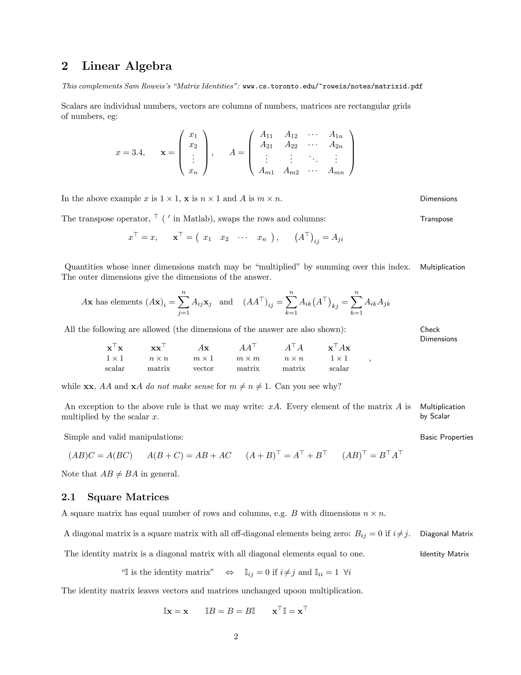
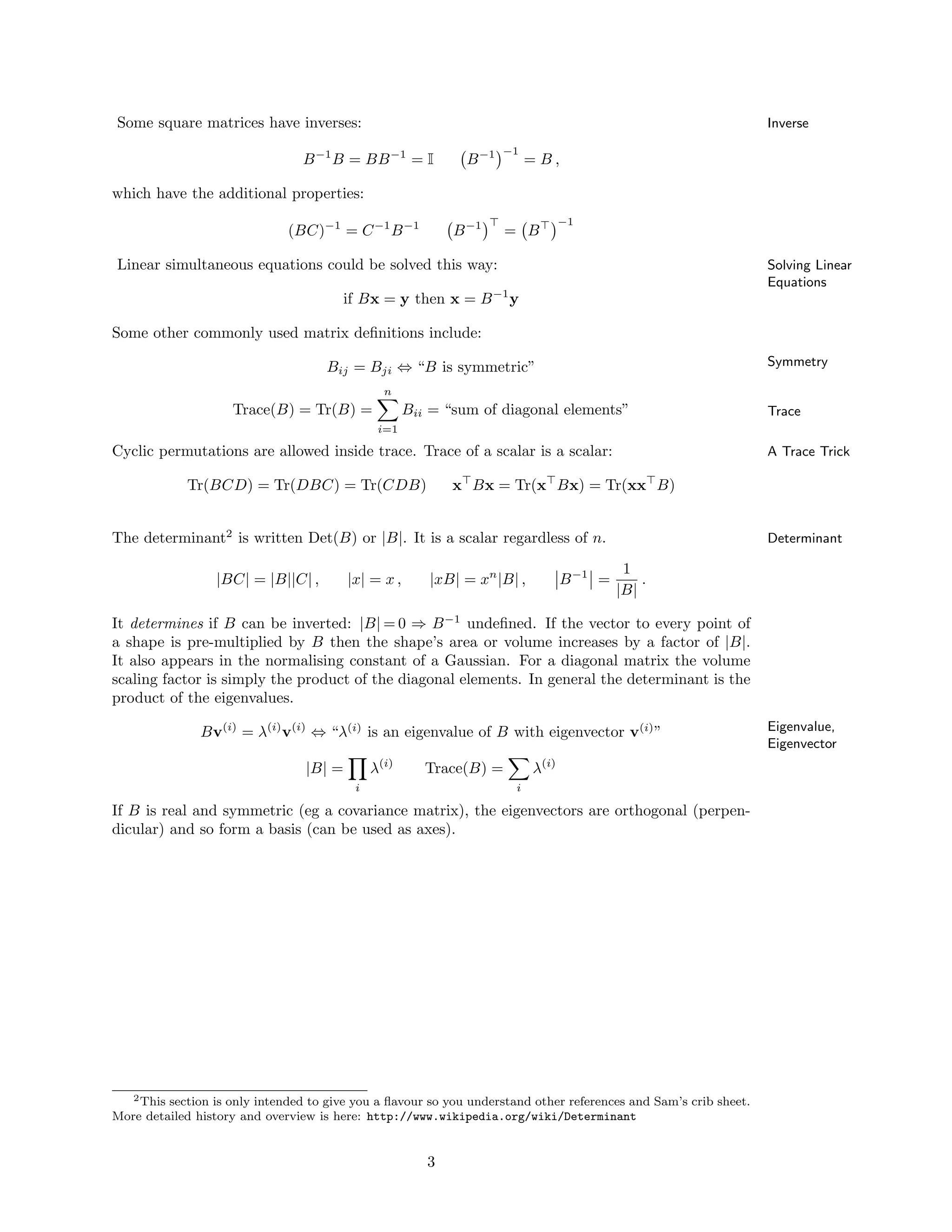
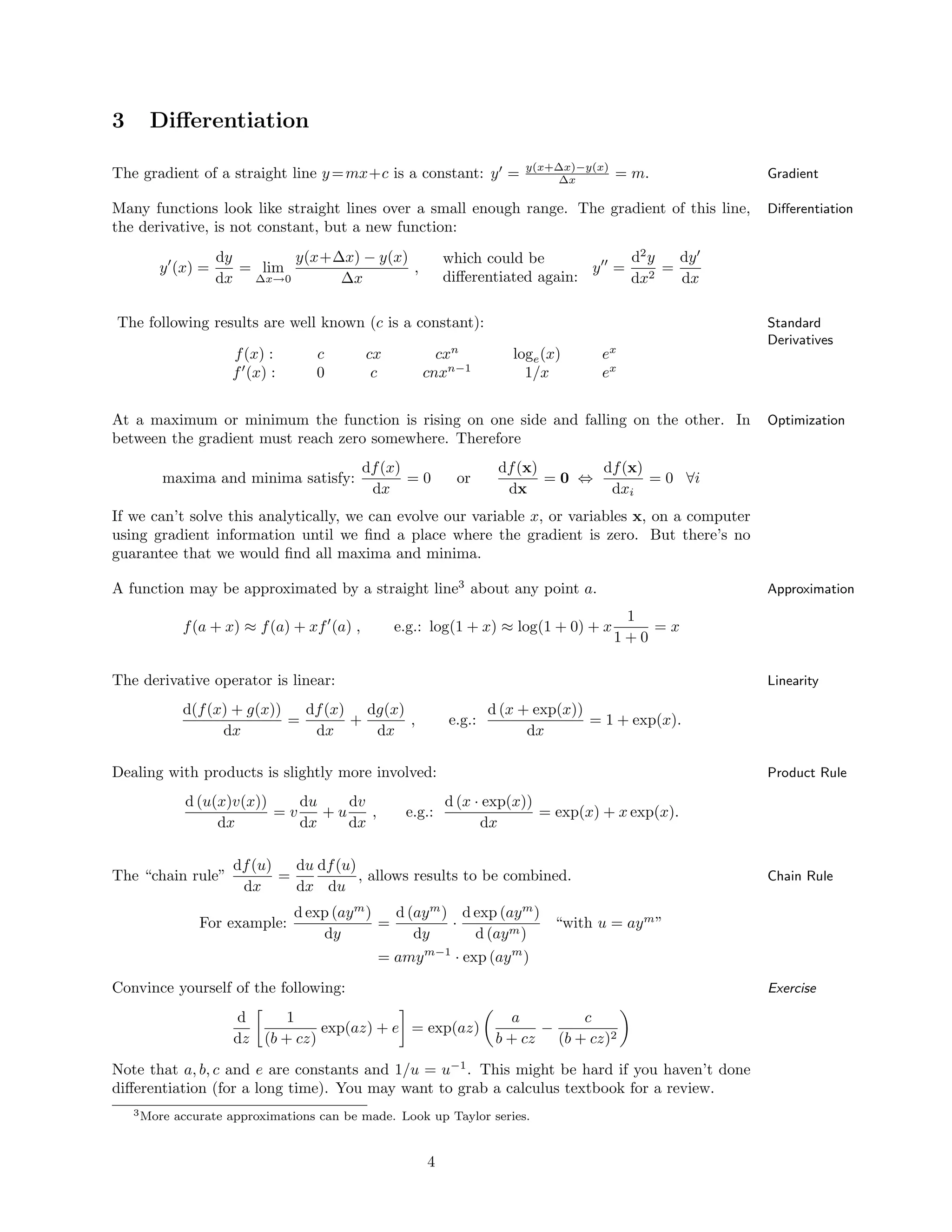
This document provides an overview of some basic mathematics concepts for machine learning, including: 1. Probability theory - definitions of probability, joint and conditional probability, Bayes' rule, expectations. 2. Linear algebra - definitions of vectors, matrices, matrix multiplication and properties, inverses, eigenvalues. 3. Differentiation - definitions of the derivative, gradient, maxima/minima, approximations, the chain rule.

1. Some Basic Mathematics for Machine Learning
Angela J. Yu <ajyu@ucsd.edu>
1 Probability Theory
See sections 2.1–2.3 of David MacKay’s book: www.inference.phy.cam.ac.uk/mackay/itila/book.html
The probability a discrete variable A takes value a is: 0 ≤ P (A=a) ≤ 1 Probability
Probabilities of alternative outcomes add: P (A∈{a, a′
}) = P (A=a) + P (A=a′
) Alternatives
The probabilities of all outcomes must sum to one:
all possible a
P (A=a) = 1 Normalization
P (A=a, B =b) is the joint probability that both A=a and B =b occur. Joint Probability
Variables can be “summed out” of joint distributions: Marginalization
P (A=a) =
all possible b
P (A=a, B =b)
P (A=a|B =b) is the probability A=a occurs given the knowledge B =b. Conditional
Probability
P (A=a, B =b) = P (A=a) P (B =b|A=a) = P (B =b) P (A=a|B =b) Product Rule
Bayes rule can be derived from the above: Bayes Rule
P (A=a|B =b, H) =
P (B =b|A=a, H) P (A=a|H)
P (B =b|H)
∝ P (A=a, B =b|H)
Marginalizing over all possible a gives the evidence or normalizing constant: Normalizing
Constant
a
P (A=a, B =b|H) = P (B =b|H)
The following hold, for all a and b, if and only if A and B are independent: Independence
P (A=a|B =b) = P (A=a)
P (B =b|A=a) = P (B =b)
P (A=a, B =b) = P (A=a) P (B =b) .
All the above theory basically still applies to continuous variables if the sums are converted Continuous
Variablesinto integrals1
. The probability that X lies between x and x+dx is p (x) dx, where p (x) is a
probability density function with range [0, ∞].
P (x1 <X <x2) =
x2
x1
p (x) dx ,
∞
−∞
p (x) dx = 1 and p (x) =
∞
−∞
p (x, y) dy.
The expectation or mean under a probability distribution is: Expectation
f(a) =
a
P (A=a) f(a) or f(x) =
∞
−∞
p (x) f(x)dx
1Integrals are the equivalent of sums for continuous variables, e.g
Pn
i=1 f(xi)∆x becomes the integral
R b
a f(x)dx in the limit ∆x → 0, n → ∞, where ∆x = b−a
n
and xi = a + i∆x.
1

2. 2 Linear Algebra
This complements Sam Roweis’s “Matrix Identities”: www.cs.toronto.edu/~roweis/notes/matrixid.pdf
Scalars are individual numbers, vectors are columns of numbers, matrices are rectangular grids
of numbers, eg:
x = 3.4, x =





x1
x2
...
xn





, A =





A11 A12 · · · A1n
A21 A22 · · · A2n
...
...
...
...
Am1 Am2 · · · Amn





In the above example x is 1 × 1, x is n × 1 and A is m × n. Dimensions
The transpose operator, ⊤
( ′
in Matlab), swaps the rows and columns: Transpose
x⊤
= x, x⊤
= x1 x2 · · · xn , A⊤
ij
= Aji
Quantities whose inner dimensions match may be “multiplied” by summing over this index. Multiplication
The outer dimensions give the dimensions of the answer.
Ax has elements (Ax)i =
n
j=1
Aijxj and (AA⊤
)ij =
n
k=1
Aik A⊤
kj
=
n
k=1
AikAjk
All the following are allowed (the dimensions of the answer are also shown): Check
Dimensions
x⊤
x
1 × 1
scalar
xx⊤
n × n
matrix
Ax
m × 1
vector
AA⊤
m × m
matrix
A⊤
A
n × n
matrix
x⊤
Ax
1 × 1
scalar
,
while xx, AA and xA do not make sense for m = n = 1. Can you see why?
An exception to the above rule is that we may write: xA. Every element of the matrix A is Multiplication
by Scalarmultiplied by the scalar x.
Simple and valid manipulations: Basic Properties
(AB)C = A(BC) A(B + C) = AB + AC (A + B)⊤
= A⊤
+ B⊤
(AB)⊤
= B⊤
A⊤
Note that AB = BA in general.
2.1 Square Matrices
A square matrix has equal number of rows and columns, e.g. B with dimensions n × n.
A diagonal matrix is a square matrix with all off-diagonal elements being zero: Bij = 0 if i=j. Diagonal Matrix
The identity matrix is a diagonal matrix with all diagonal elements equal to one. Identity Matrix
“I is the identity matrix” ⇔ Iij = 0 if i=j and Iii = 1 ∀i
The identity matrix leaves vectors and matrices unchanged upoon multiplication.
Ix = x IB = B = BI x⊤
I = x⊤
2

3. Some square matrices have inverses: Inverse
B−1
B = BB−1
= I B−1 −1
= B ,
which have the additional properties:
(BC)−1
= C−1
B−1
B−1 ⊤
= B⊤ −1
Linear simultaneous equations could be solved this way: Solving Linear
Equations
if Bx = y then x = B−1
y
Some other commonly used matrix definitions include:
SymmetryBij = Bji ⇔ “B is symmetric”
TraceTrace(B) = Tr(B) =
n
i=1
Bii = “sum of diagonal elements”
Cyclic permutations are allowed inside trace. Trace of a scalar is a scalar: A Trace Trick
Tr(BCD) = Tr(DBC) = Tr(CDB) x⊤
Bx = Tr(x⊤
Bx) = Tr(xx⊤
B)
The determinant2
is written Det(B) or |B|. It is a scalar regardless of n. Determinant
|BC| = |B||C| , |x| = x , |xB| = xn
|B| , B−1
=
1
|B|
.
It determines if B can be inverted: |B| = 0 ⇒ B−1
undefined. If the vector to every point of
a shape is pre-multiplied by B then the shape’s area or volume increases by a factor of |B|.
It also appears in the normalising constant of a Gaussian. For a diagonal matrix the volume
scaling factor is simply the product of the diagonal elements. In general the determinant is the
product of the eigenvalues.
Eigenvalue,
Eigenvector
Bv(i)
= λ(i)
v(i)
⇔ “λ(i)
is an eigenvalue of B with eigenvector v(i)
”
|B| =
i
λ(i)
Trace(B) =
i
λ(i)
If B is real and symmetric (eg a covariance matrix), the eigenvectors are orthogonal (perpen-
dicular) and so form a basis (can be used as axes).
2This section is only intended to give you a flavour so you understand other references and Sam’s crib sheet.
More detailed history and overview is here: http://www.wikipedia.org/wiki/Determinant
3

4. 3 Differentiation
The gradient of a straight line y=mx+c is a constant: y′
= y(x+∆x)−y(x)
∆x = m. Gradient
Many functions look like straight lines over a small enough range. The gradient of this line, Differentiation
the derivative, is not constant, but a new function:
y′
(x) =
dy
dx
= lim
∆x→0
y(x+∆x) − y(x)
∆x
,
which could be
differentiated again:
y′′
=
d2
y
dx2
=
dy′
dx
The following results are well known (c is a constant): Standard
Derivatives
f(x) :
f′
(x) :
c
0
cx
c
cxn
cnxn−1
loge(x)
1/x
ex
ex
At a maximum or minimum the function is rising on one side and falling on the other. In Optimization
between the gradient must reach zero somewhere. Therefore
maxima and minima satisfy:
df(x)
dx
= 0 or
df(x)
dx
= 0 ⇔
df(x)
dxi
= 0 ∀i
If we can’t solve this analytically, we can evolve our variable x, or variables x, on a computer
using gradient information until we find a place where the gradient is zero. But there’s no
guarantee that we would find all maxima and minima.
A function may be approximated by a straight line3
about any point a. Approximation
f(a + x) ≈ f(a) + xf′
(a) , e.g.: log(1 + x) ≈ log(1 + 0) + x
1
1 + 0
= x
The derivative operator is linear: Linearity
d(f(x) + g(x))
dx
=
df(x)
dx
+
dg(x)
dx
, e.g.:
d (x + exp(x))
dx
= 1 + exp(x).
Dealing with products is slightly more involved: Product Rule
d (u(x)v(x))
dx
= v
du
dx
+ u
dv
dx
, e.g.:
d (x · exp(x))
dx
= exp(x) + x exp(x).
The “chain rule”
df(u)
dx
=
du
dx
df(u)
du
, allows results to be combined. Chain Rule
For example:
d exp (aym
)
dy
=
d (aym
)
dy
·
d exp (aym
)
d (aym)
“with u = aym
”
= amym−1
· exp (aym
)
Convince yourself of the following: Exercise
d
dz
1
(b + cz)
exp(az) + e = exp(az)
a
b + cz
−
c
(b + cz)2
Note that a, b, c and e are constants and 1/u = u−1
. This might be hard if you haven’t done
differentiation (for a long time). You may want to grab a calculus textbook for a review.
3More accurate approximations can be made. Look up Taylor series.
4