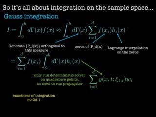
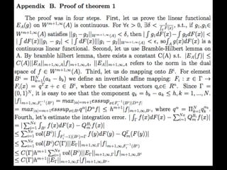
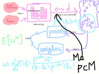
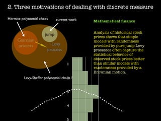
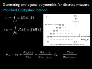
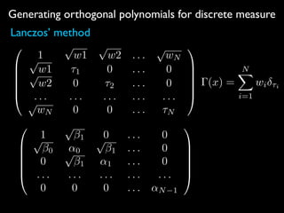
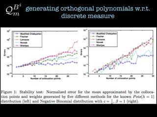
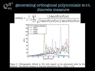
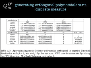
This document summarizes research on computing stochastic partial differential equations (SPDEs) using an adaptive multi-element polynomial chaos method (MEPCM) with discrete measures. Key points include: 1) MEPCM uses polynomial chaos expansions and numerical integration to compute SPDEs with parametric uncertainty. 2) Orthogonal polynomials are generated for discrete measures using various methods like Vandermonde, Stieltjes, and Lanczos. 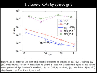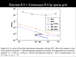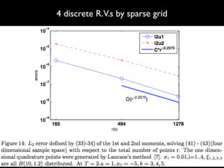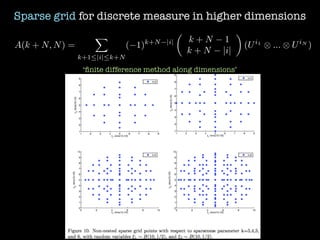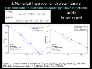3) Numerical integration is tested on discrete measures using Genz functions in 1D and sparse grids in higher dimensions. 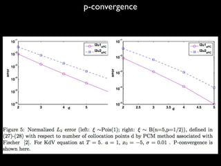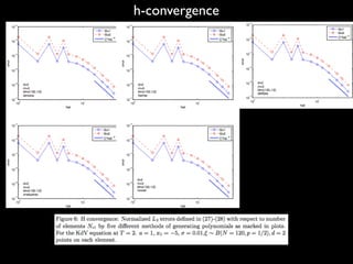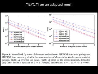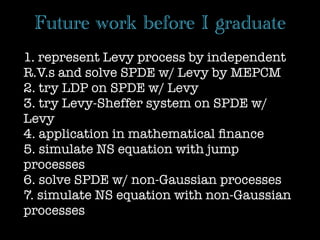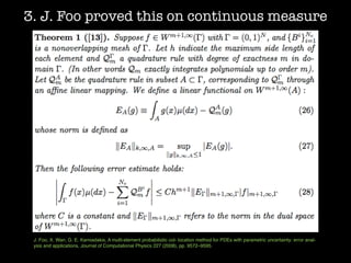4) The method is demonstrated on the KdV equation with random initial conditions. Future work includes applying these techniques to SPDEs driven

1. Adaptive multi-element polynomial chaos with
discrete measure: Algorithms and application to
SPDEs
Mengdi Zheng and George Karniadakis

2. Content:
1. computing SPDE by MEPCM
2. motivations
3. numerical integration on discrete
measure
4. numerical example on KdV
equation
5. future work

3. 1.What computational SPDE is about? (MEPCM)
Xt(!) E[y(x, t; !)]
Xt(!)
Xt(⇠1, ⇠2, ...⇠n)
...
⇠n
⇠3
⇠2
⇠1
⌦
E[ym
(x, t; !)]
E[ym
(x, t; ⇠1, ⇠2, ..., ⇠n)]
fix x, t, integration
over a finite
dimensional
sample space
MEPCM=FEM on
sample space
⇠1
⇠2
⌦
⇡ ⇡
Gauss quadratures

4. So it’s all about integration on the sample space...
Gauss integration
I =
Z b
a
d (x)f(x) ⇡
Z b
a
d (x)
dX
i=1
f(xi)hi(x)
=
dX
i=1
f(xi)
Z b
a
d (x)hi(x)
Generate {P_i(x)} orthogonal to
this measure
zeros of P_d(x) Lagrange interpolation
on the zeros
dX
i=1
y(x, t; ⇠1,i)wi
only run deterministic solver
on quadrature points,
no need to run propagator
exactness of integration
m=2d-1

5. 2. Three motivations of dealing with discrete measure
Gaussian
process Levy
process
Hermite polynomial chaos
Levy-Sheffer polynomial chaos ?
jump
current work
Analysis of historical stock
prices shows that simple
models with randomness
provided by pure jump Levy
processes often capture the
statistical behavior of
observed stock prices better
than similar models with
randomness provided by a
Brownian motion.
Mathematical finance
1
2
3
4
5

6. 3. J. Foo proved this on continuous measure
J. Foo, X. Wan, G. E. Karniadakis, A multi-element probabilistic col- location method for PDEs with parametric uncertainty: error anal-
ysis and applications, Journal of Computational Physics 227 (2008), pp. 9572–9595.

7. 3. Can we prove it on discrete measure?
for discrete measure
" =
NX
i=1
i⌘"
⌧i
,
lim
"!0
⌘"
⌧i
= ⌧i , lim
"!0
" = .
Z
f(x) (dx)
NeX
i=1
QBi
m f 
Z
f(x) (dx)
Z
f(x) "(dx)
+
Z
f(x) "(dx)
NeX
i=1
Q",Bi
m f +
NeX
i=1
Q",Bi
m f
NeX
i=1
QBi
m f ,
h / N 1
es N (m+1)
es
m = 2d 1
N 2d
es
=
NX
i=1
i ⌧i ⌦
⌧1 ⌧2 ⌧3

10. Generating orthogonal polynomials for discrete measure
Vandermonde matrix method
µk =
Z
R
xk
(dx)
0
B
B
B
B
@
µ0 µ1 . . . µk
µ1 µ2 . . . µk+1
. . . . . . . . . . . .
µk 1 µk . . . µ2k 1
0 0 . . . 1
1
C
C
C
C
A
0
B
B
B
B
@
p0
p1
. . .
pk 1
pk
1
C
C
C
C
A
=
0
B
B
B
B
@
0
0
. . .
0
1
1
C
C
C
C
A

11. Generating orthogonal polynomials for discrete measure
Stieltjes’ method
↵i =
R
R
xP2
i (x) (dx)
R
R
P2
i (x) (dx)
, i =
R
R
xP2
i (x) (dx)
R
R
P2
i 1(x) (dx)
Pj+1(x) = (x ↵j)Pj(x) jPj 1(x) j = 1, . . .

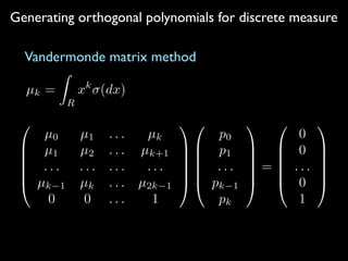
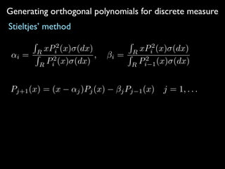
12. Generating orthogonal polynomials for discrete measure
Fischer’s method
=
NX
i=1
i ⌧i ⌫ = + ⌧
↵⌫
i = ↵i +
2
i Pi(⌧)Pi+1(⌧)
1 +
Pi
j=0
2
j P2
j (⌧)
2
i 1Pi(⌧)Pi 1(⌧)
1 +
Pi 1
j=0
2
j P2
j (⌧)
⌫
i = i
[1 +
Pi 2
j=0
2
j P2
j (⌧)][1 +
Pi
j=0
2
j P2
j (⌧)]
[1 +
Pi 1
j=0
2
j P2
j (⌧)]2

13. Generating orthogonal polynomials for discrete measure
Modified Chebyshev method
⌫r =
Z
⌦
pr(⇠)d (⇠)
kl =
Z
⌦
Pk(⇠)pl(⇠)d (⇠)
↵k = ak +
k,k+1
kk
k 1,k
k 1,k 1
, k =
k,k
k 1,k 1

14. Generating orthogonal polynomials for discrete measure
Lanczos’ method
0
B
B
B
B
@
1
p
w1
p
w2 . . .
p
wNp
w1 ⌧1 0 . . . 0p
w2 0 ⌧2 . . . 0
. . . . . . . . . . . . . . .
p
wN 0 0 . . . ⌧N
1
C
C
C
C
A
0
B
B
B
B
@
1
p
1 0 . . . 0p
0 ↵0
p
1 . . . 0
0
p
1 ↵1 . . . 0
. . . . . . . . . . . . . . .
0 0 0 . . . ↵N 1
1
C
C
C
C
A
(x) =
NX
i=1
wi ⌧i

15. QBi
m
generating orthogonal polynomials w.r.t.
discrete measure

16. QBi
m
generating orthogonal polynomials w.r.t.
discrete measure

17. QBi
m
generating orthogonal polynomials w.r.t.
discrete measure

18. 3. Numerical integration on discrete measure
test theorem on discrete measure by GENZ functions
in 1D

19. 3. Numerical integration on discrete measure
in 1D
test theorem on discrete measure by GENZ functions

20. Sparse grid for discrete measure in higher dimensions
A(k + N, N) =
X
k+1|i|k+N
( 1)k+N |i|
✓
k + N 1
k + N |i|
◆
(Ui1
⌦ ... ⌦ UiN
)
‘finite difference method along dimensions’

21. 3. Numerical integration on discrete measure
in 2D
by sparse grid
test theorem on discrete measure by GENZ functions

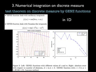
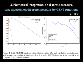
22. Numerical example on KdV equation
ut + 6uux + uxxx = ⇠, x 2 R
u(x, 0) =
a
2
sech2
(
p
a
2
(x x0))
< um
(x, T; !) >=
Z
R
d⇢(⇠)[
a
2
sech2
(
p
a
2
(x 3 ⇠T2
x0 aT)) + ⇠T]m
L2u1 =
qR
dx(E[unum(x, T; !)] E[uex(x, T; !)])2
qR
dx(E[uex(x, T; !)])2
L2u2 =
qR
dx(E[u2
num(x, T; !)] E[u2
ex(x, T; !)])2
qR
dx(E[u2
ex(x, T; !)])2

23. p-convergence

24. h-convergence

25. MEPCM on an adapted mesh
⇠1
⇠2
⌦
Gauss quadratures
Criterion:
divide integration
domain s.t. we minimize
the difference in
variance
‘local variance’ criterion

26. MEPCM on an adapted mesh

27. 2 discrete R.V.s by sparse grid

28. Discrete R.V. + Continuous R.V. by sparse grid

29. 4 discrete R.V.s by sparse grid

30. Future work before I graduate
1. represent Levy process by independent
R.V.s and solve SPDE w/ Levy by MEPCM
2. try LDP on SPDE w/ Levy
3. try Levy-Sheffer system on SPDE w/
Levy
4. application in mathematical finance
5. simulate NS equation with jump
processes
6. solve SPDE w/ non-Gaussian processes
7. simulate NS equation with non-Gaussian
processes