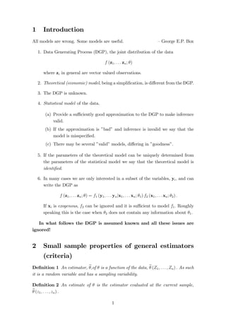
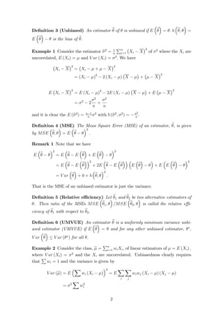
1. The document discusses statistical estimation and properties of estimators such as bias, variance, consistency, and asymptotic normality. 2. Key concepts covered include unbiasedness, mean squared error, relative efficiency, sufficiency, and properties of estimators like consistency, asymptotic unbiasedness, and best asymptotic normality. 3. Examples are provided to illustrate theoretical estimators for parameters like the variance of a distribution or coefficients in a linear regression model.

1. Lecture notes Statistics
Estimation
Rickard Sandberg e-mail:rickard.sandberg@hhs.se
January 22, 2010

2. 1 Introduction
All models are wrong. Some models are useful. –George E.P. Box
1. Data Generating Process (DGP), the joint distribution of the data
f (z1; : : : zn; )
where zi in general are vector valued observations.
2. Theoretical (economic) model, being a simpli…cation, is di¤erent fromthe DGP.
3. The DGP is unknown.
4. Statistical model of the data.
(a) Provide a su¢ ciently good approximation to the DGP to make inference
valid.
(b) If the approximation is ”bad” and inference is invalid we say that the
model is misspeci…ed.
(c) There may be several ”valid”models, di¤ering in ”goodness”.
5. If the parameters of the theoretical model can be uniquely determined from
the parameters of the statistical model we say that the theoretical model is
identi…ed.
6. In many cases we are only interested in a subset of the variables, yi; and can
write the DGP as
f (z1; : : : zn; ) = f1 (y1; : : : ynjx1; : : : xn; 1) f2 (x1; : : : xn; 2) :
If xi is exogenous, f2 can be ignored and it is su¢ cient to model f1: Roughly
speaking this is the case when 2 does not contain any information about 1.
In what follows the DGP is assumed known and all these issues are
ignored!
2 Small sample properties of general estimators
(criteria)
De…nition 1 An estimator, b;of is a function of the data, b (Z1; : : : ;Zn) : As such
it is a random variable and has a sampling variability.
De…nition 2 An estimate of is the estimator evaluated at the current sample,
b (z1; : : : ; zn) :
1

3. De…nition 3 (Unbiased) An estimator b of is unbiased if E
b
= : b
b;
=
E
b
is the bias of b:
Example 1 Consider the estimator b2 = 1
n
Pn
i=1
Xi X
2 of 2 where the Xi are
uncorrelated, E (Xi) = and V ar (Xi) = 2: We have
Xi X
2
=
Xi + X
2
= (Xi )2 2 (Xi )
X
+
X
2
E
Xi X
2
= E (Xi )2 2E (Xi )
X
+ E
X
2
= 2 2
2
n
+
2
n
n 2 with b (b2; 2) = 2
and it is clear the E (b2) = n1
n :
De…nition 4 (MSE) The Mean Square Error (MSE) of an estimator, b;
is given
by MSE
b;
= E
b
2
:
Remark 1 Note that we have
E
b
2
= E
b E
b
+ E
b
2
= E
b E
b
2
+ 2E
b E
b
E
b
+ E
E
b
2
= V ar
b
+ 0 + b
b;
2
:
That is the MSE of an unbiased estimator is just the variance.
De…nition 5 (Relative e¢ ciency) Let b1 and b2 be two alternative estimators of
. Then ratio of the MSEs MSE
b1;
=MSE
b2;
is called the relative e¢ -
ciency of b1 with respect to b2:
De…nition 6 (UMVUE) An
estimator b is a uniformly minimum variance unbi-
ased estimator (UMVUE) if E
b
= and for any other unbiased estimator, ;
V ar
b
V ar () for all :
Example 2 Consider the class, b =
Pn
i=1 wiXi, of linear estimators of = E (Xi) ;
where 2 and the are uncorrelated. Unbiasedness clearly requires
P
V ar (Xi) = Xi that
wi = 1 and the variance is given by
V ar (b) = E
X
2
wi (Xi )
= E
X
i
X
j
wiwj (Xi ) (Xj )
= 2
X
w2
i
2

4. One unbiased estimator in this class is the familiar X which sets wi = 1=n and has
variance 2=n:We will show that this is the UMVUE in the class of linear estimators.
P
The …rst order condition for minimizing V ar (b) subject to the restriction
wi = 1
is
2wi =
for the Lagrange multiplier. That is, all the weights are equal, together with
P
wi = 1 this gives wi = 1=n:
Remark 2 The notion of minimizing the variance is suggestive. One can de…ne
a general class of estimators by requiring the estimator to minimize the sample
analogue of the variance
b = arg min n1
Xn
i=1
(Xi )2 ;
with FOC 2n1Pn
i=1 (Xi ) = 0 and solution b = 1
n
P
Xi: This is the class of
Least Squares estimators.
Example 3 Consider the linear regression model
yi =

5. 1 + x2i

6. 2 + : : : + xki

7. k + i
or in matrix notation
y = X

8. + :
The least squares estimator of

9. ; b; is obtained byminimizing q = 0 = (y Xb)0 (y Xb).
The FOC is
@q
@b0
= 2 (y Xb)0X = 0
y0X = b0X0X
with solution
b = (X0X)1X0y
provided that X0X has full rank (so the inverse is well-de…ned), i.e. that X has rank
k:
Theorem 1 (Gauss-Markov) Assume that X is non-stochastic and E () = 0;
V ar () = 2I: Then V ar (b) = 2 (X0X)1 and b is the BLUE (Best Linear Un-
biased Estimator) of

10. : That is, b is the UMVUE in the class of linear estimators,
eb
= Ay:
Proof. Write
b = (X0X)1X0y =(X0X)1X0 (X

11. + ) =

12. + (X0X)1X0:
3

13. This immediately gives E (b) =

14. and
V ar (b) = E (b

15. ) (b

16. )0 = E
h
(X0X)1X00X(X0X)1
i
= (X0X)1X0E (0)X(X0X)1 = (X0X)1X02IX (X0X)1
= 2 (X0X)1 :
To prove that b is BLUE, let= Ay be an unbiased linear estimator of

17. : De…ning
C eb
= A(X0X)1X0 we have=
C + (X0X)1X0
y = Cy+b = CX

18. +C +

19. +
eb
(X0X)1X0: Clearly
E
eb
= CX

20. + CE () +

21. = CX

22. +

23. and unbiasedness implies that CX = 0: The variance is then
V ar
eb
= E
eb

24. eb

25. 0 = E
h
C+(X0X)1X0
i
0
h
C+(X0X)1X0
i
0
= 2CC0 + 2CX(X0X)1 + 2 (X0X)1X0C + 2 (X0X)1
= 2CC0 + 2 (X0X)1
and the variance of eb
exceeds the variance of b by the positive semi-de…nite matrix
2CC0: This implies that V ar
0eb
= V ar (0b) + 20CC0 V ar (0b) for any
linear combination :
De…nition 7 (Su¢ ciency) Let f (x; ) be the joint density of the data. T (x) is
said to be a su¢ cient statistic for if g (xjT) ; the density of x conditional on T
does not depend on :
Remark 3 A su¢ cient statistic T captures all the information about in the data.
This means that we can base estimators on T rather than the full sample.
Theorem 2 (Factorization theorem) Let X1; :::;Xn be a random sample from
f (x; ). Then T(x) is su¢ cient statistic for i¤
f (x; ) = g (x) f (T(x); )
where g does not depend on :
Example 4 Let Xi be iid Bernoulli with parameter p. T =
Pn
i=1 Xi is then a
su¢ cient statistic (i.e. the number of successes in n trials). The joint pdf is given
by
f (x;p) =
Yn
i=1
pxi (1 p)1xi = p
P
xi (1 p)n
P
xi = g (xjT) h (T; ) :
and we can put g (x) = 1 and f (T; p) = pT (1 p)nT with T =
Pn
i=1 Xi.
Remark 4 Note that su¢ cient statistics are not unique and may di¤er in how
P
good they are at reducing the data. In the previous example T2 = n
Xi and
T3 = (
P
Xi; n
P
Xi) are clearly su¢ cient statistics as well.
4