Downloaded 33 times


Bayesian statistics uses probability to represent uncertainty about unknown parameters in statistical models. It differs from classical statistics in that parameters are treated as random variables rather than fixed unknown constants. Bayesian probability represents a degree of belief in an event rather than the physical probability of an event. The Bayes' formula provides a way to update beliefs based on new evidence or data using conditional probability. Bayesian networks are graphical models that compactly represent joint probability distributions over many variables and allow for efficient inference.
Introduction to the theme of Bayesian statistics.
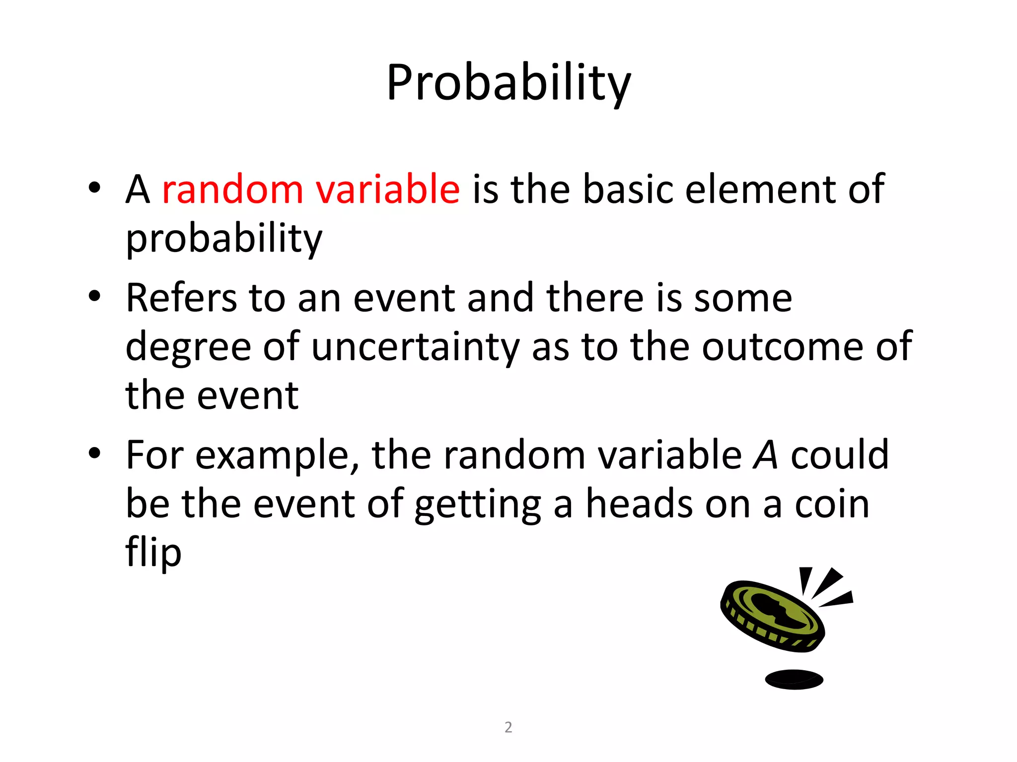
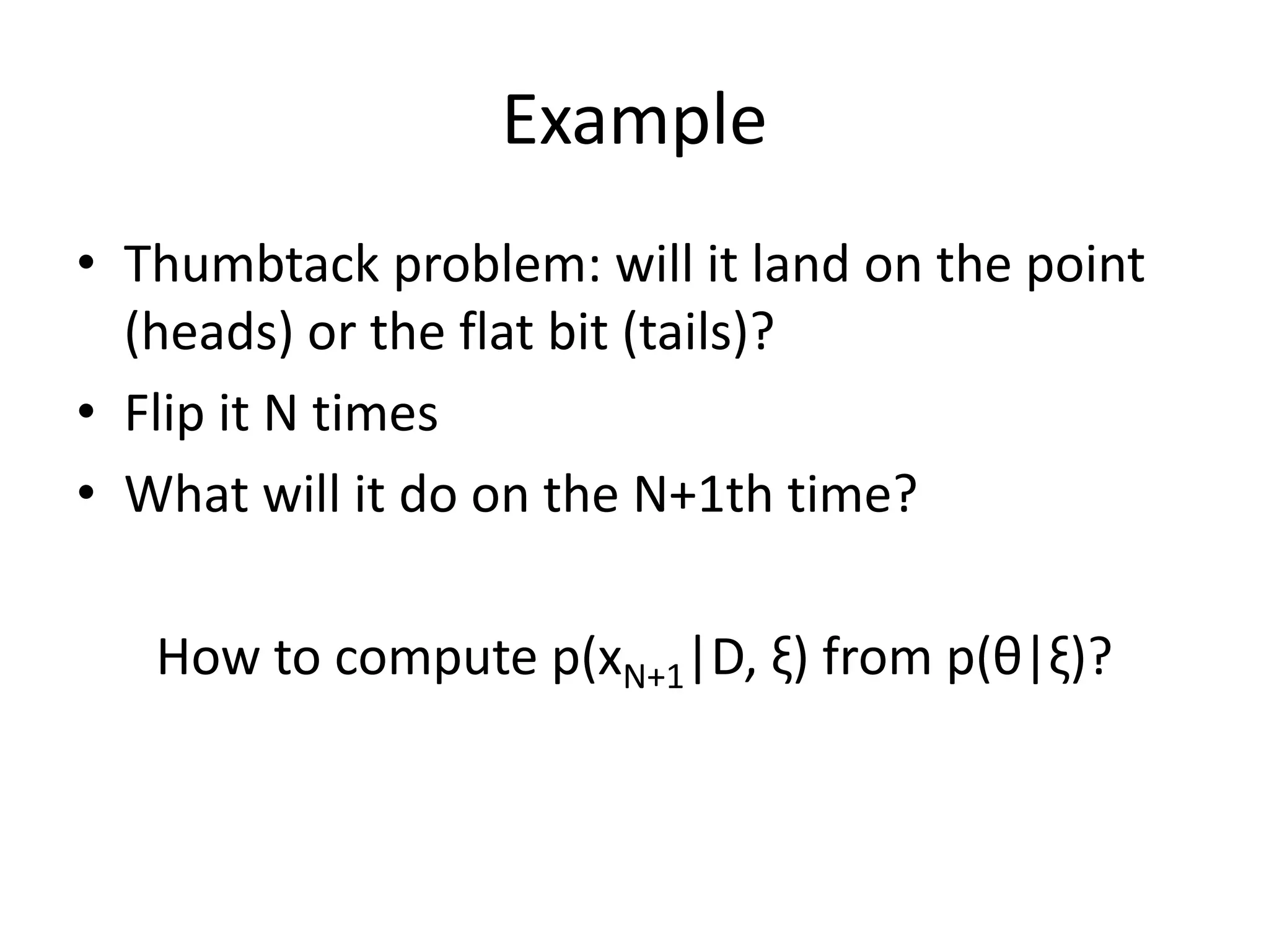
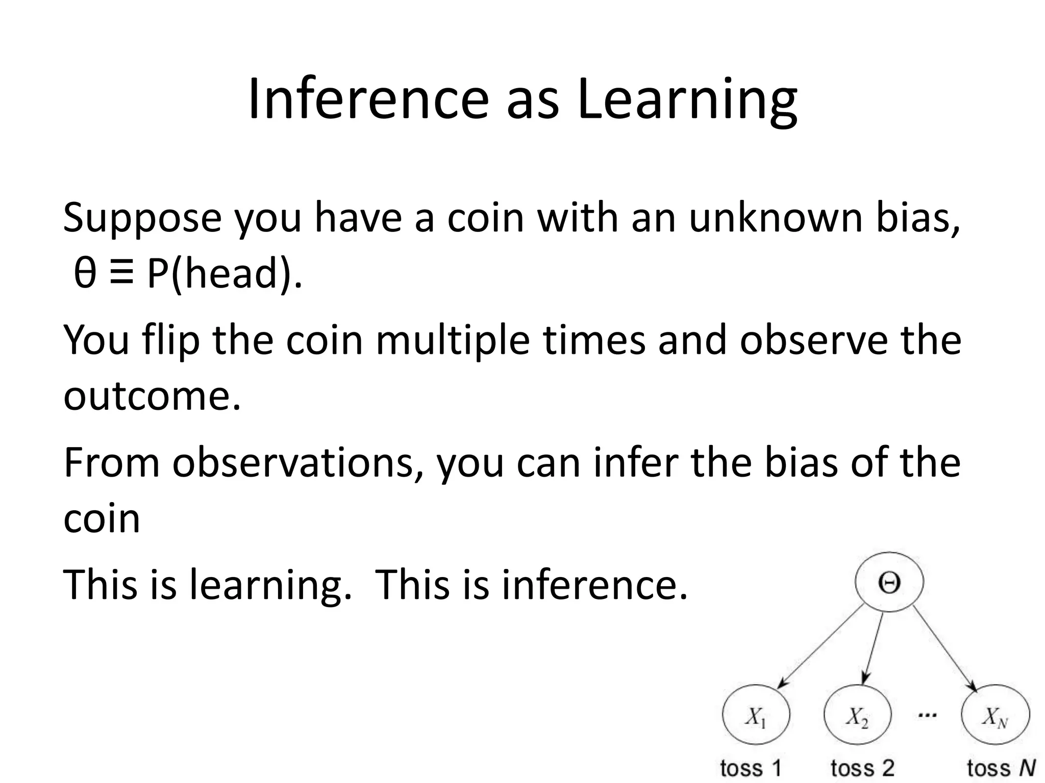
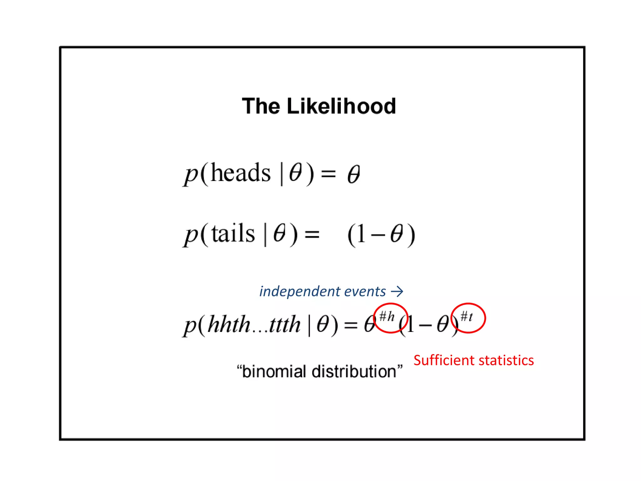
Covers concepts of random variables and uncertainty, exemplified with coin flips.
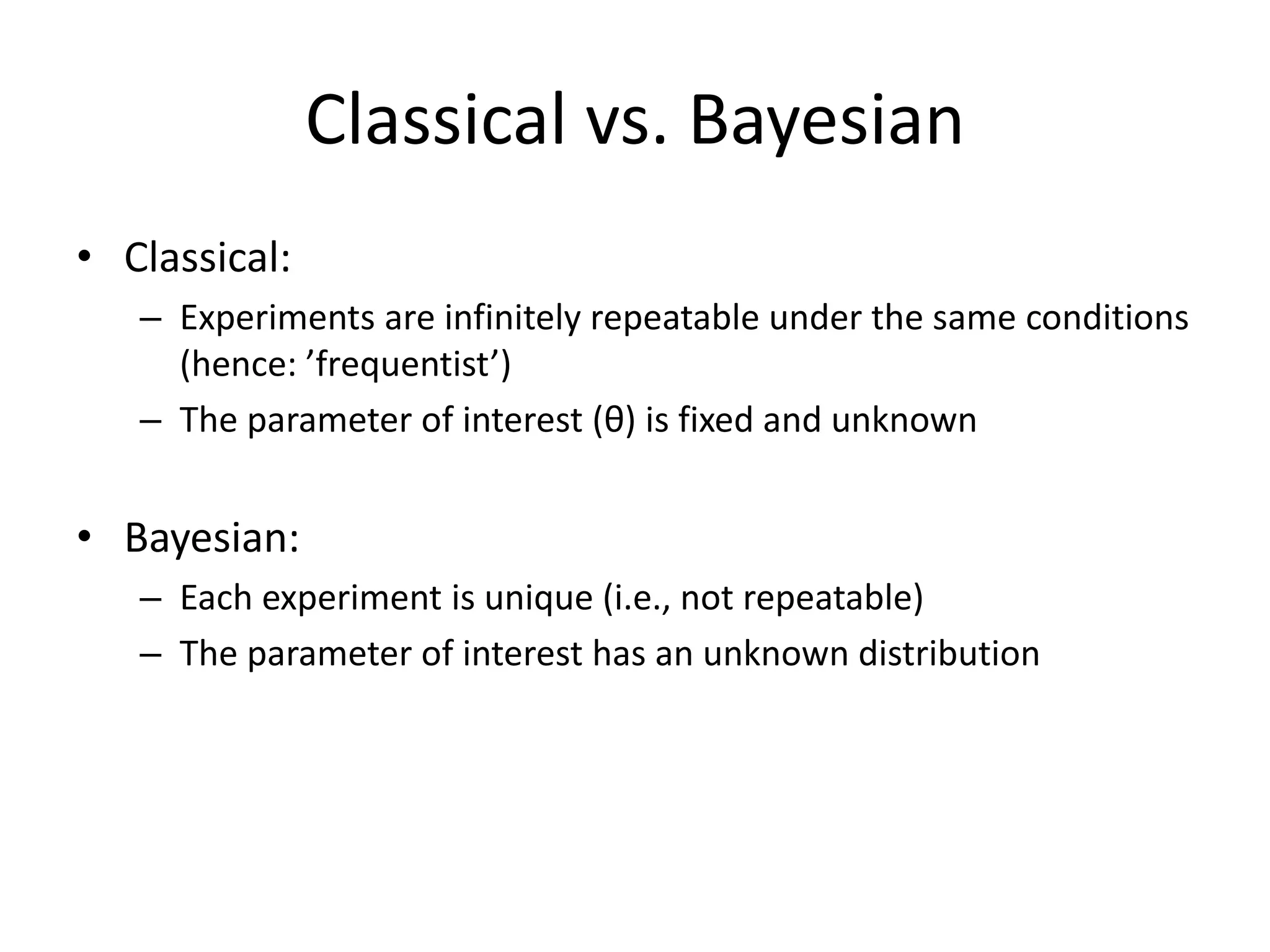
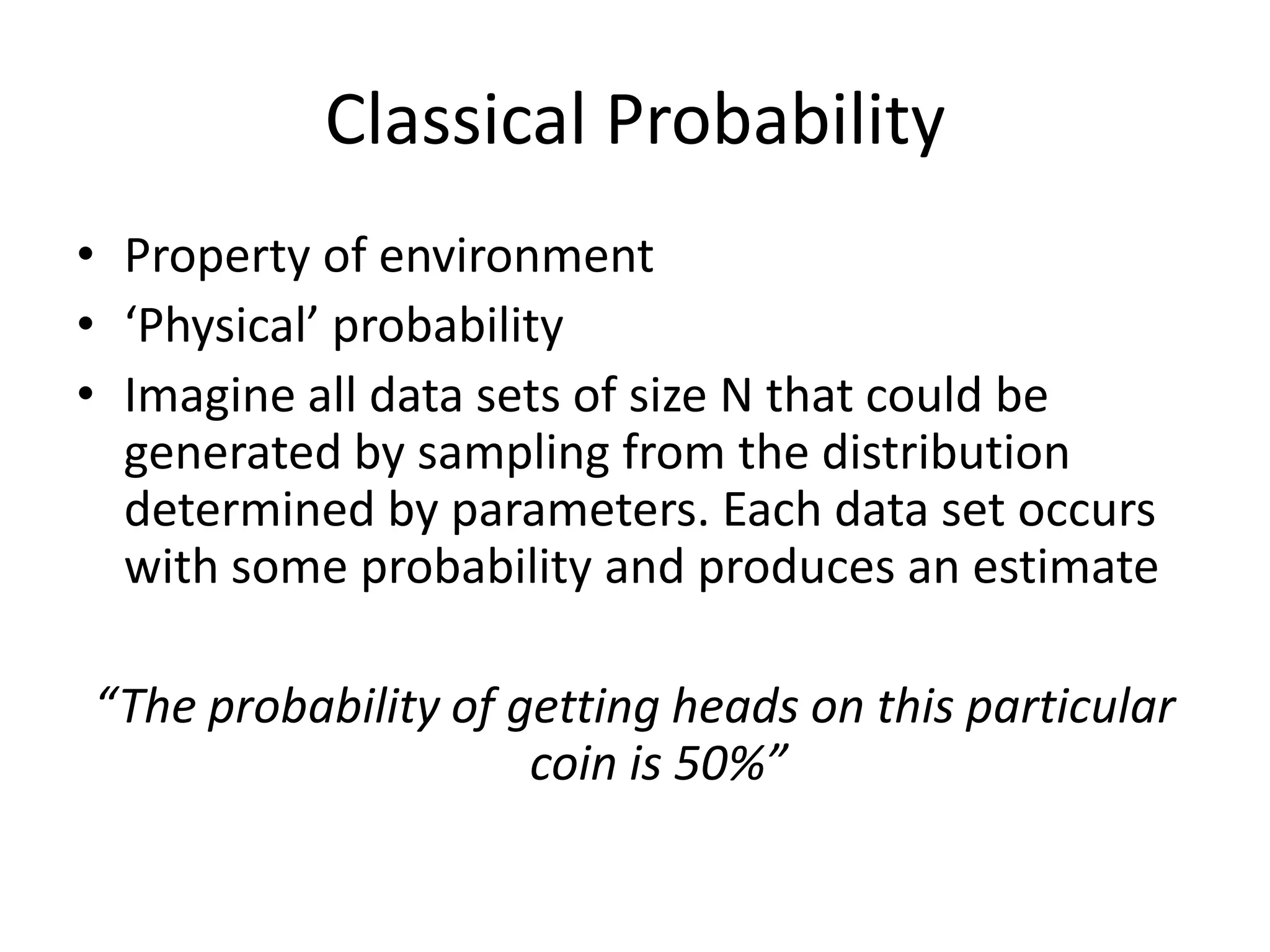
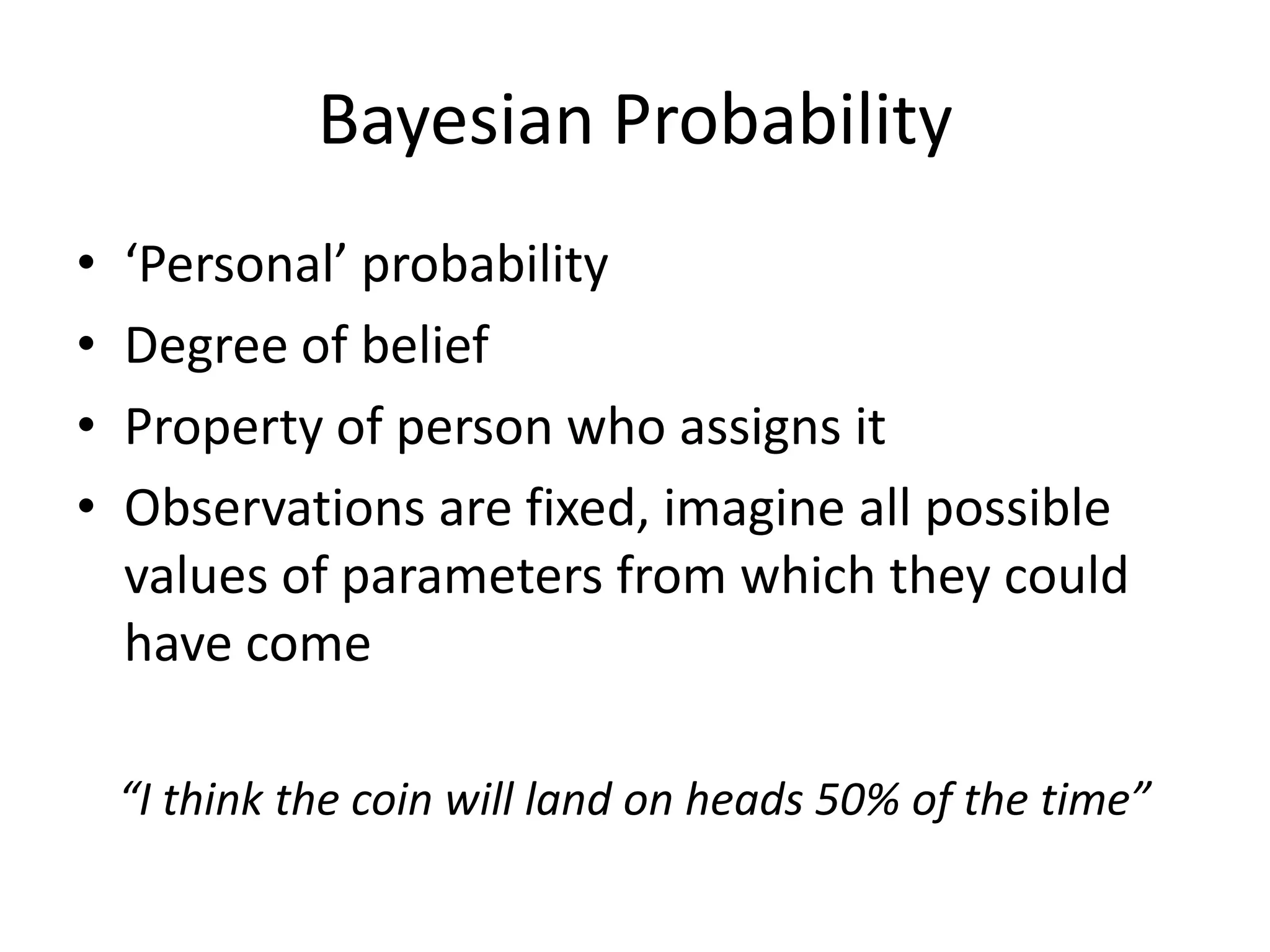
Contrasts classical and Bayesian probability with definitions and characteristics.
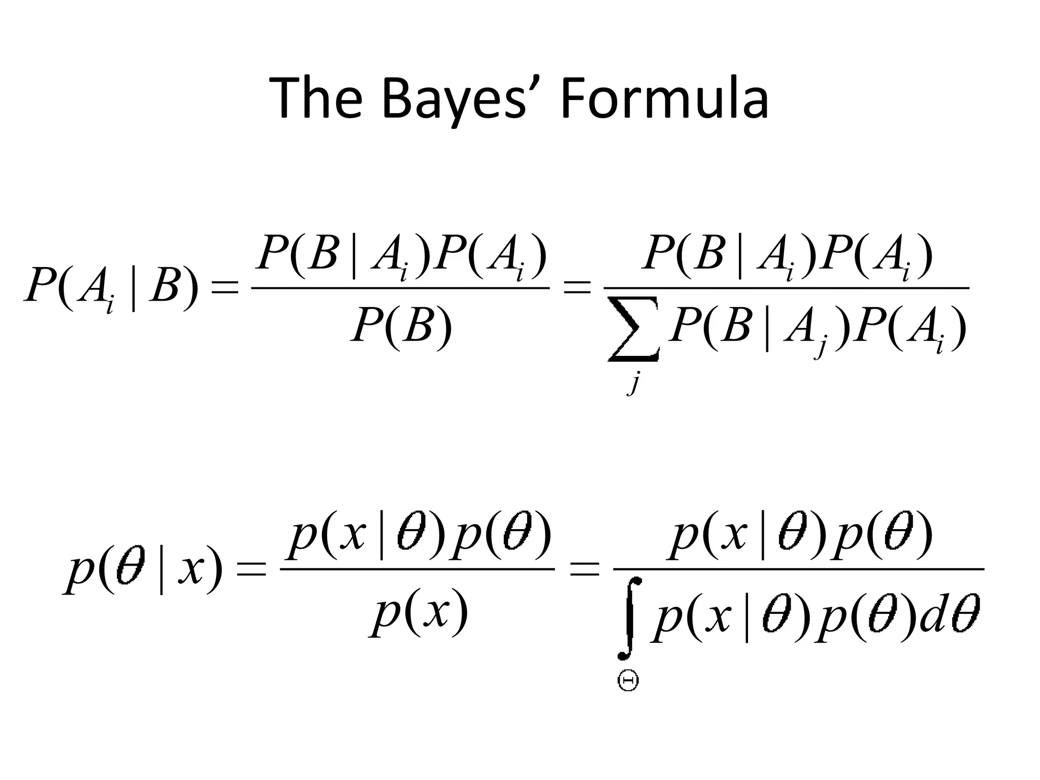
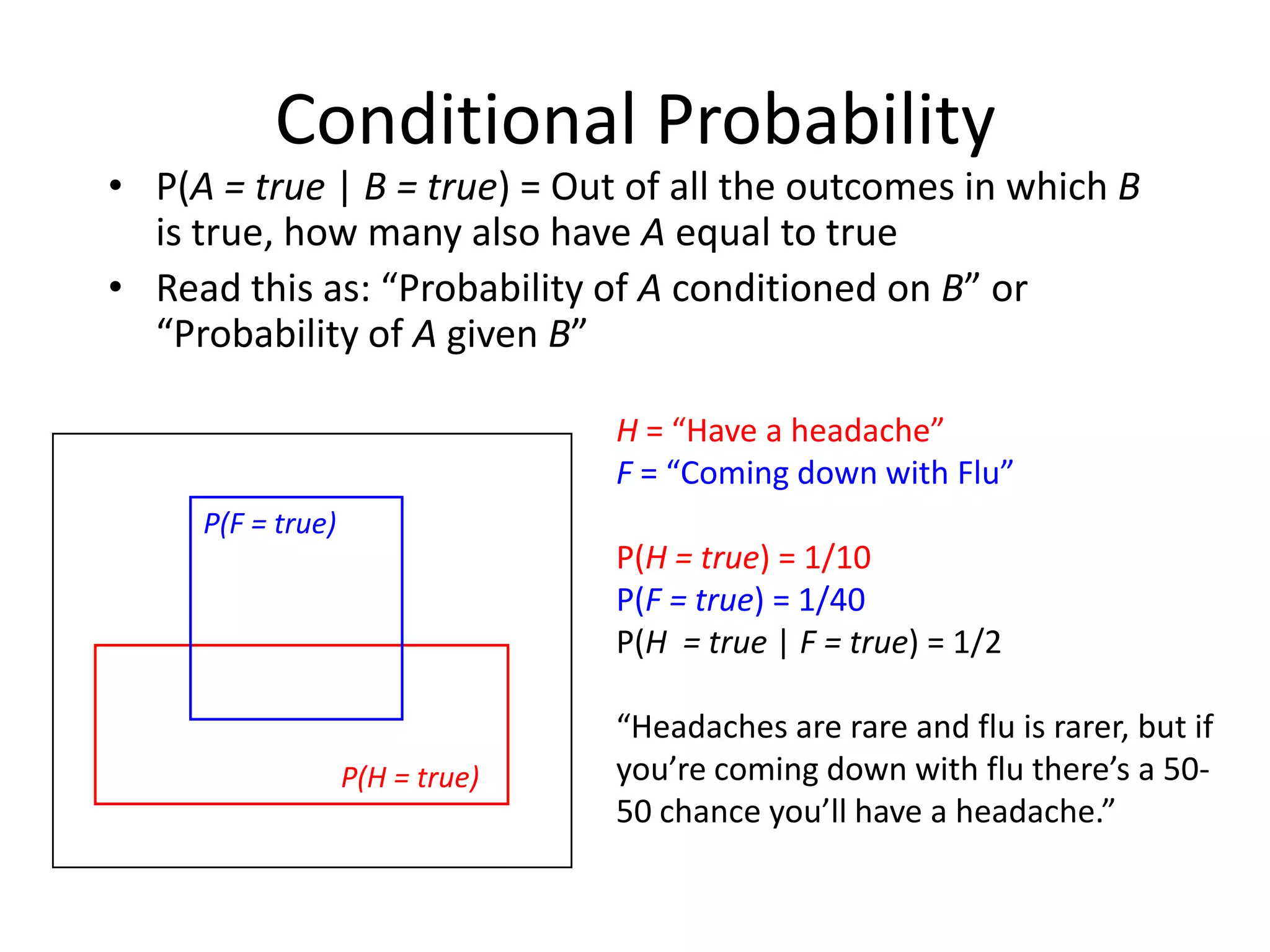
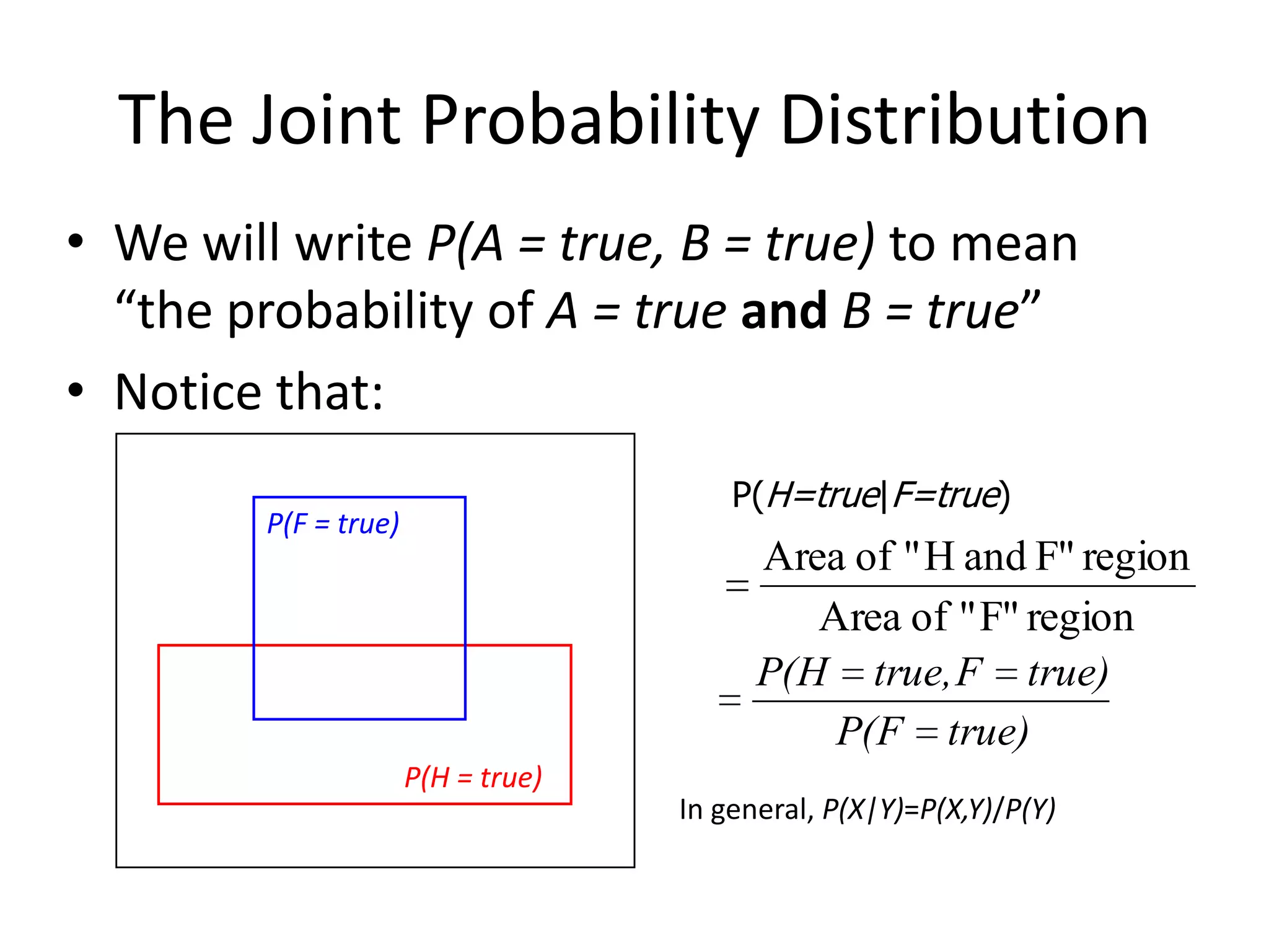
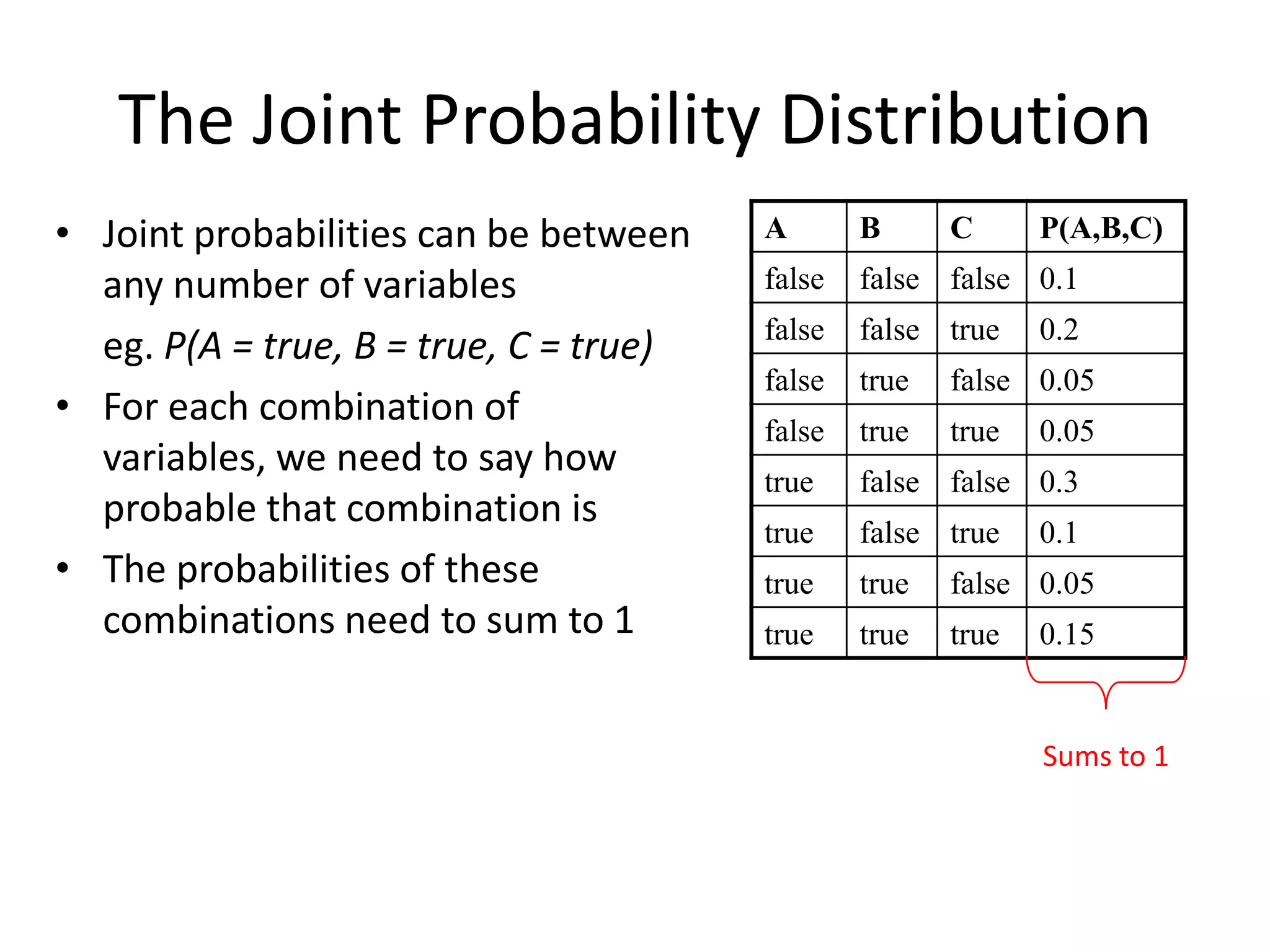
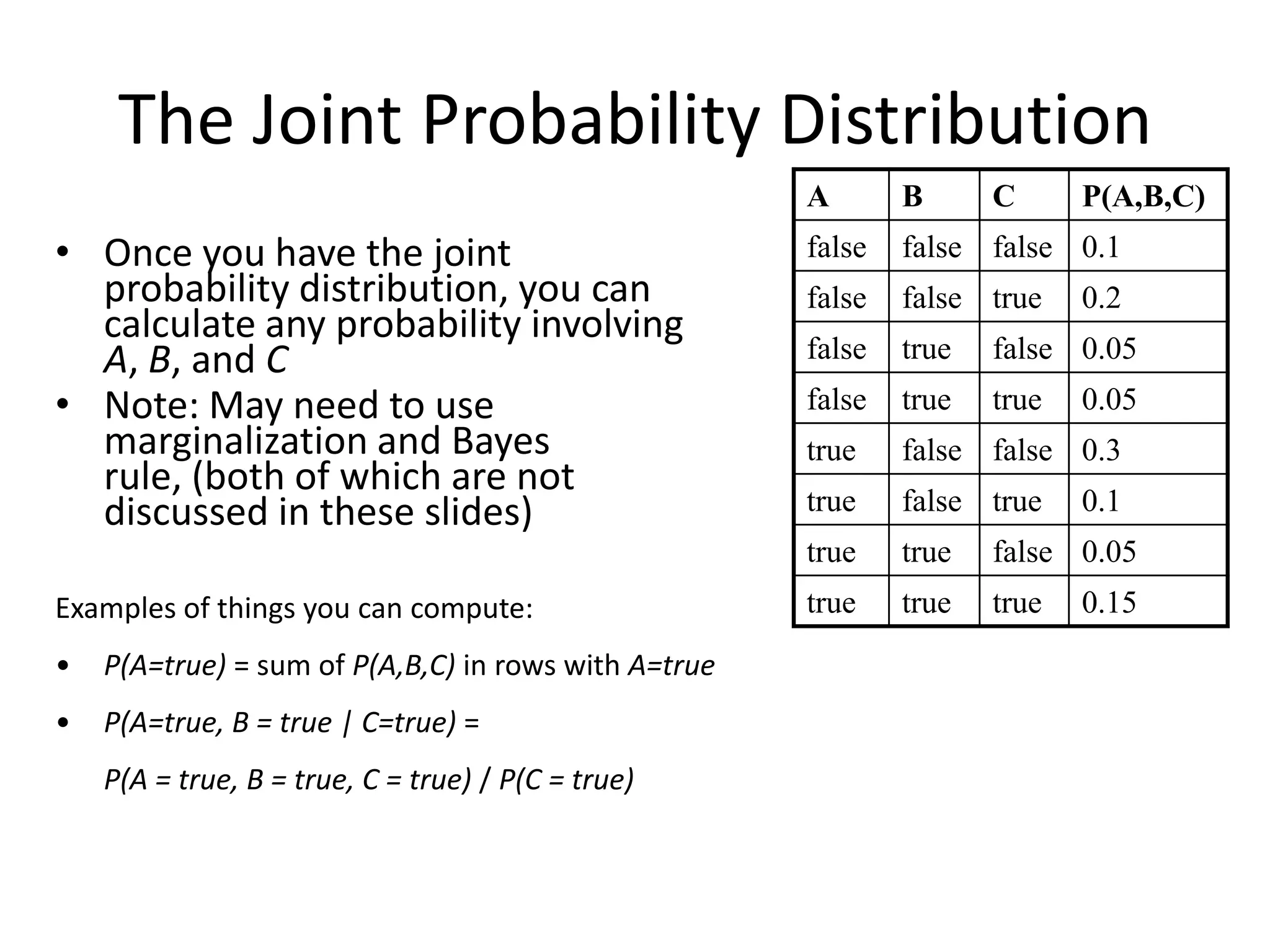
Introduction to Bayes' formula, conditional probability, and joint probability distribution.
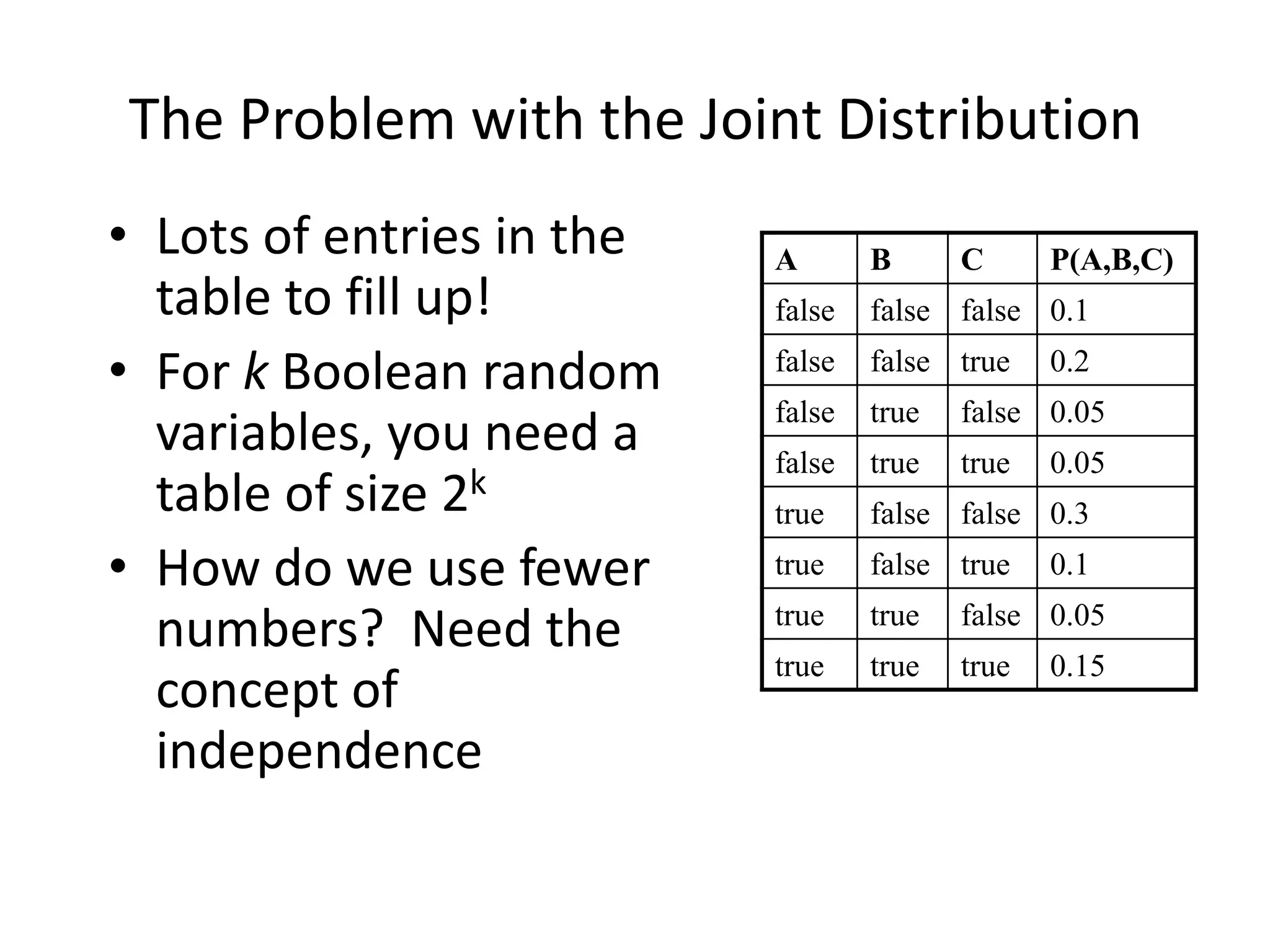
Discusses complexity in joint distributions and the importance of independence.
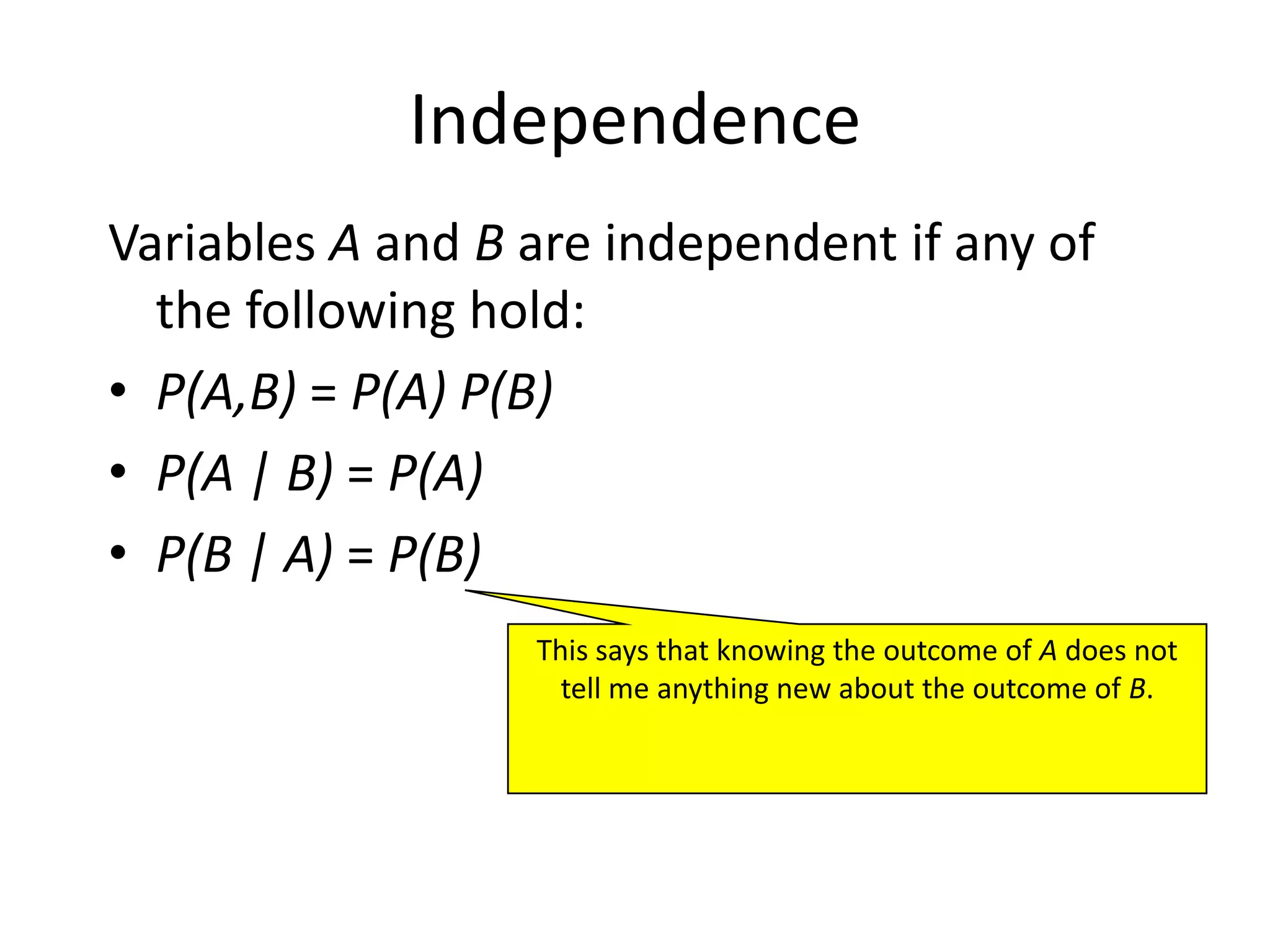
Definition and implications of independence in random variables.
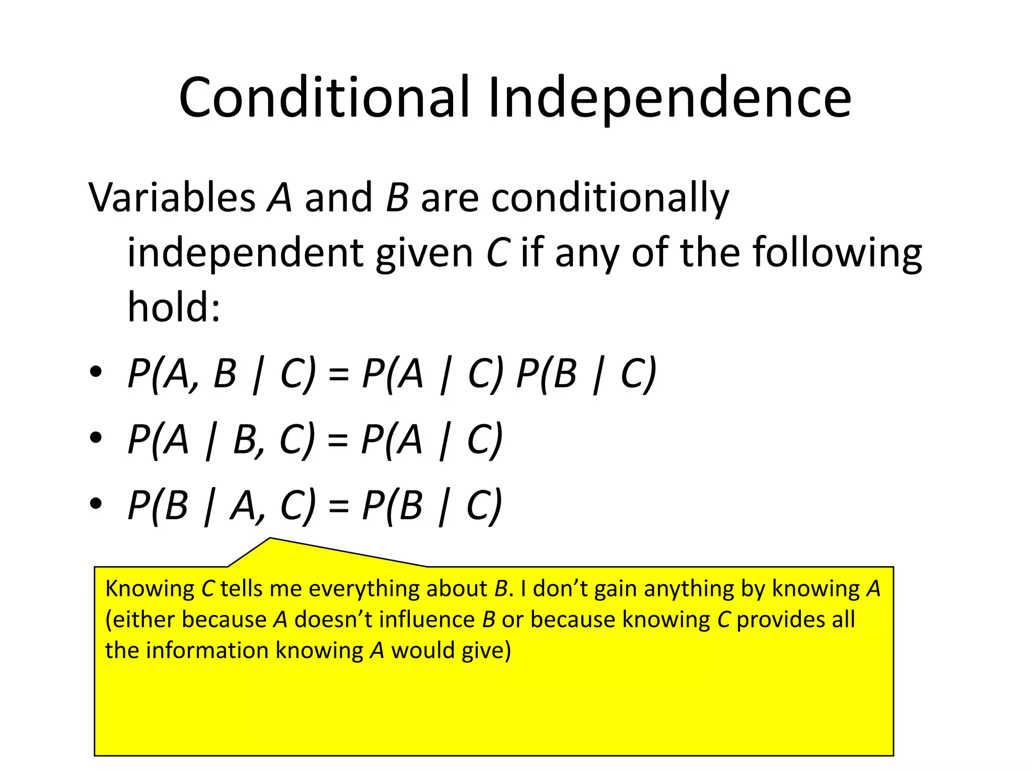
Explains conditional independence and its significance in probability assessments.
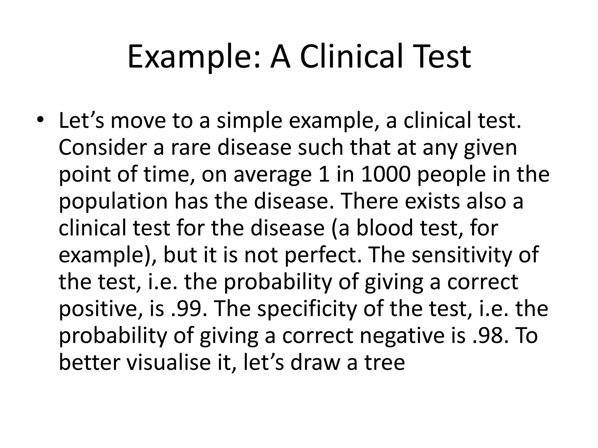
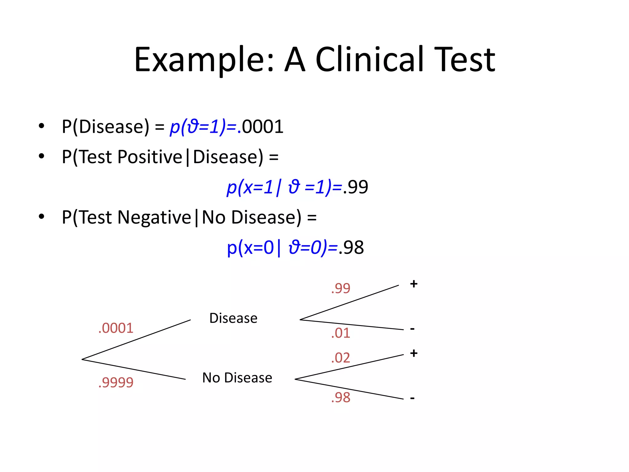
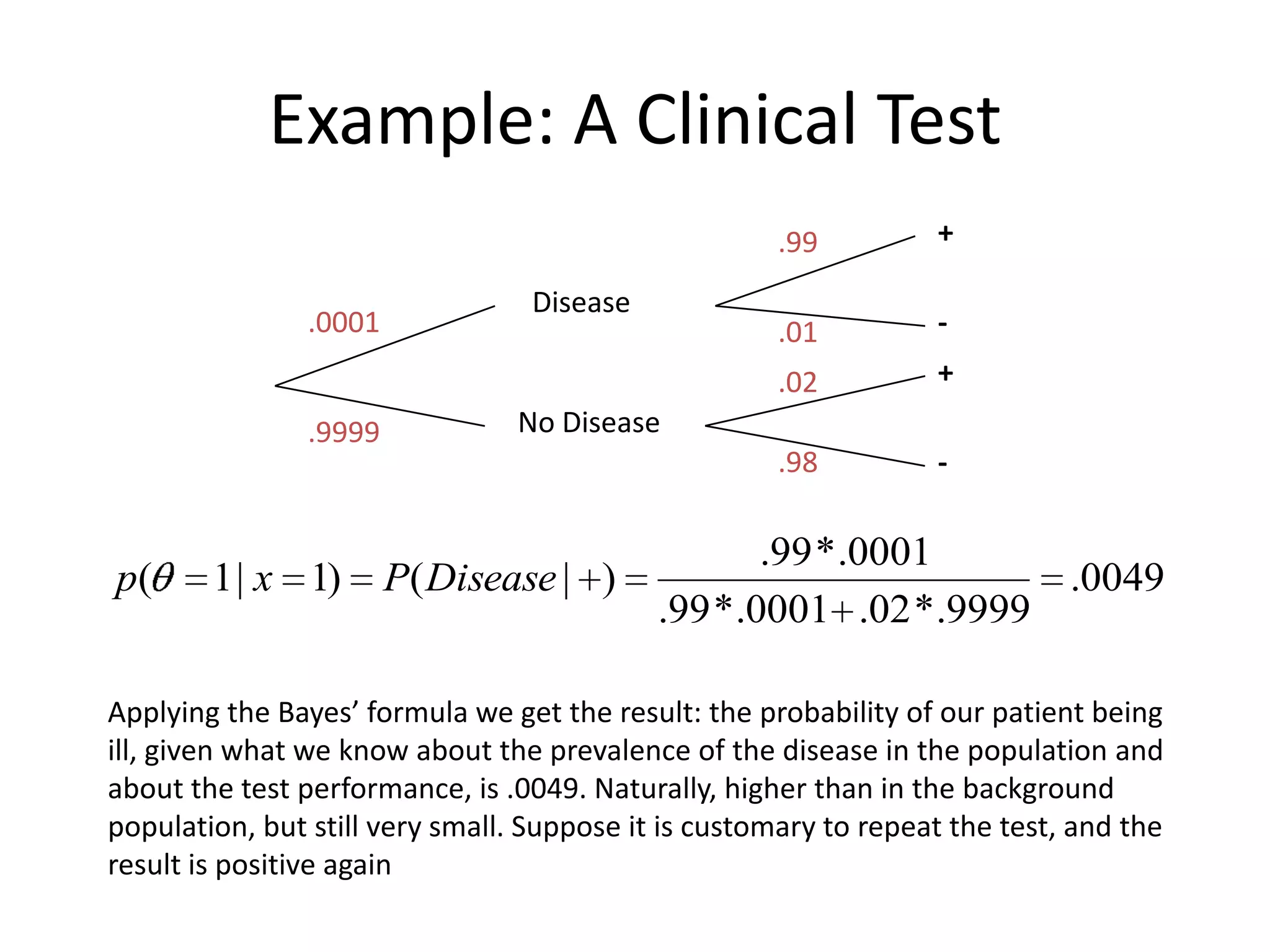
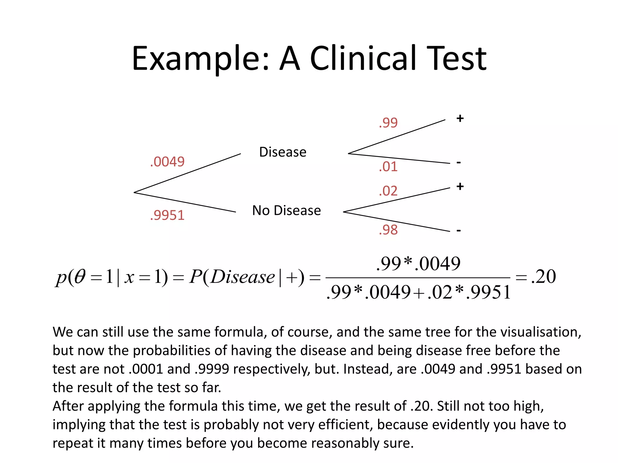
Application of Bayesian principles to a clinical test involving a rare disease.
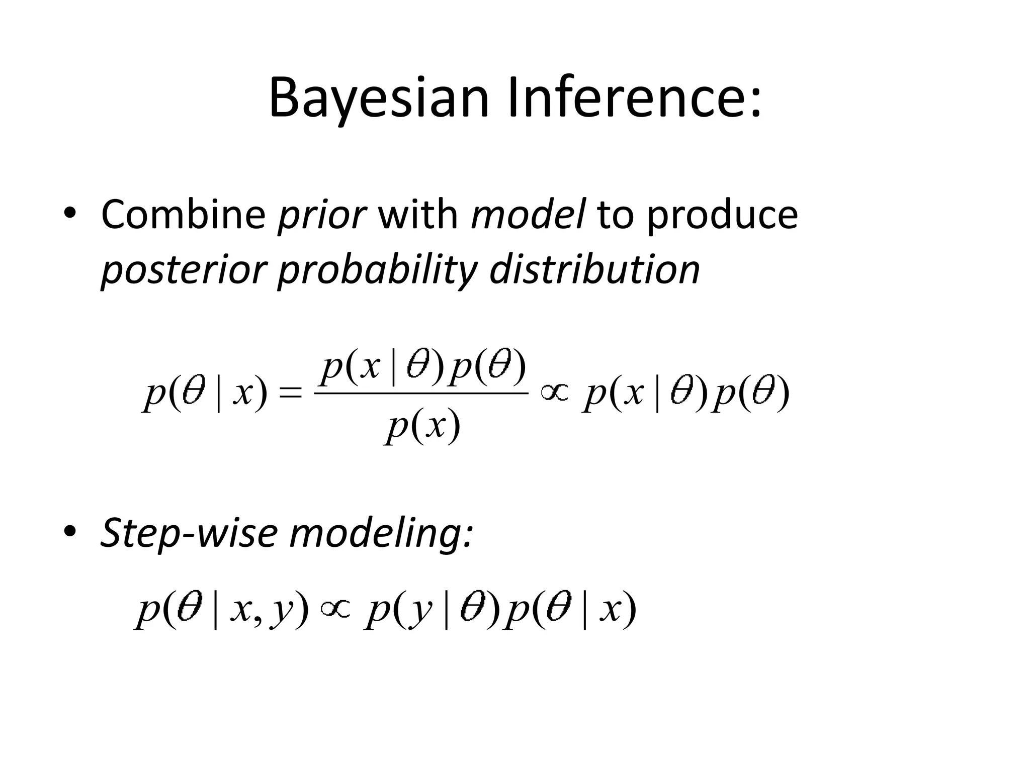
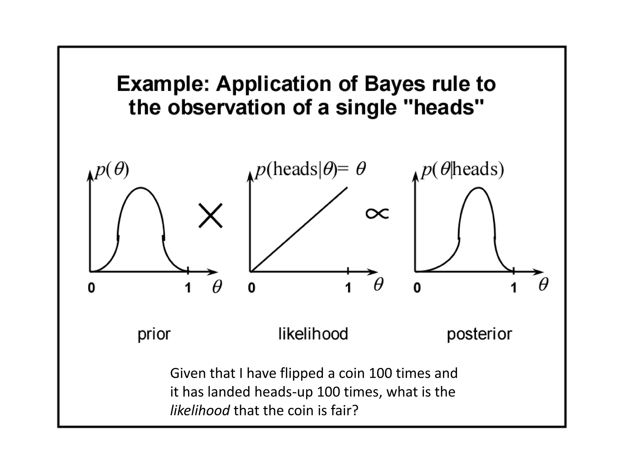
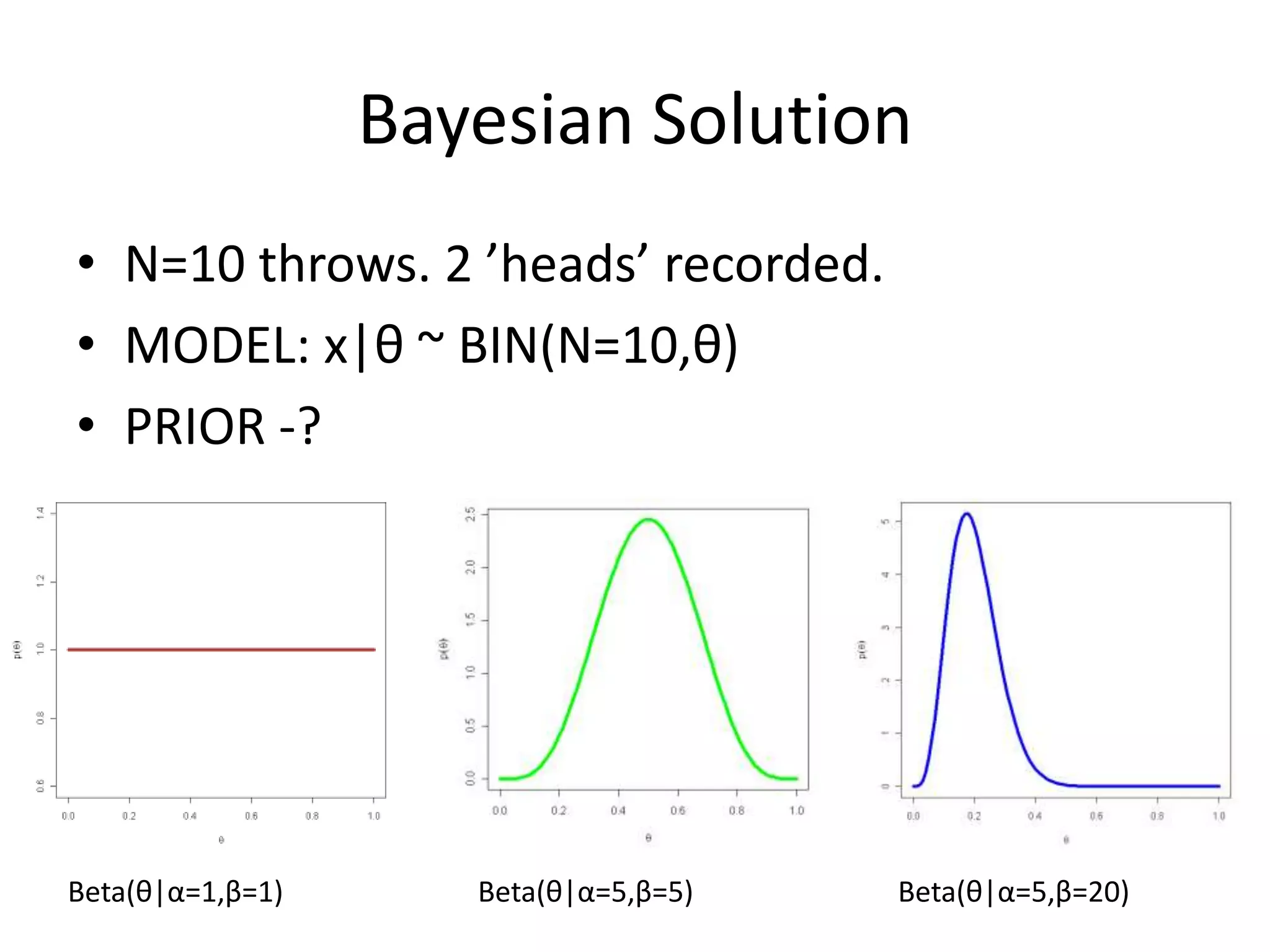
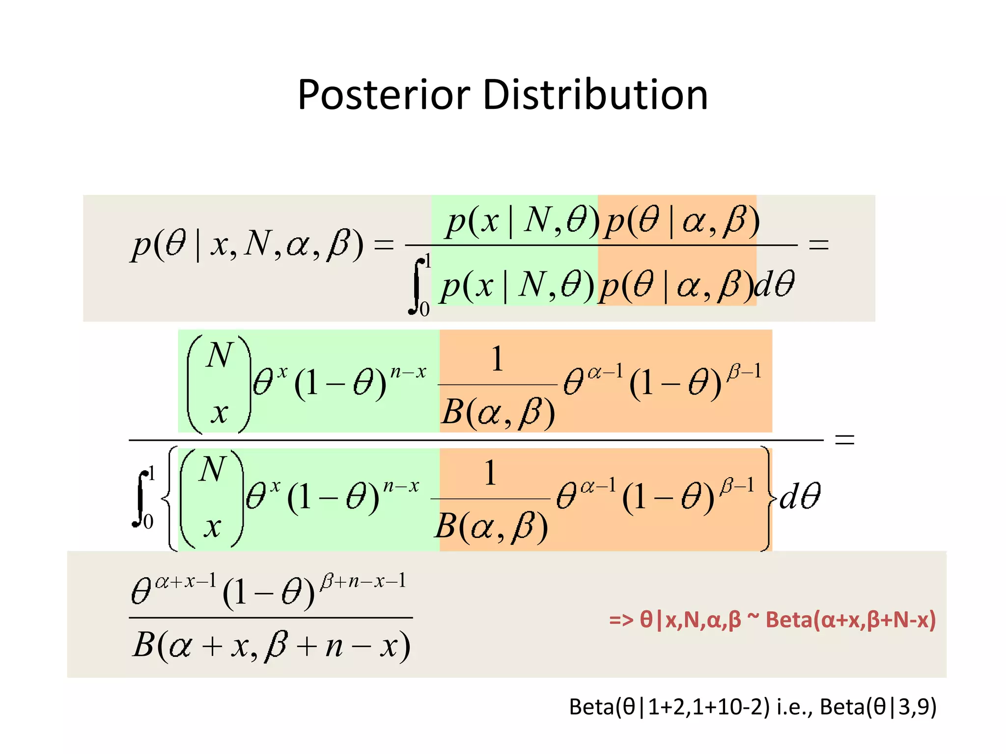
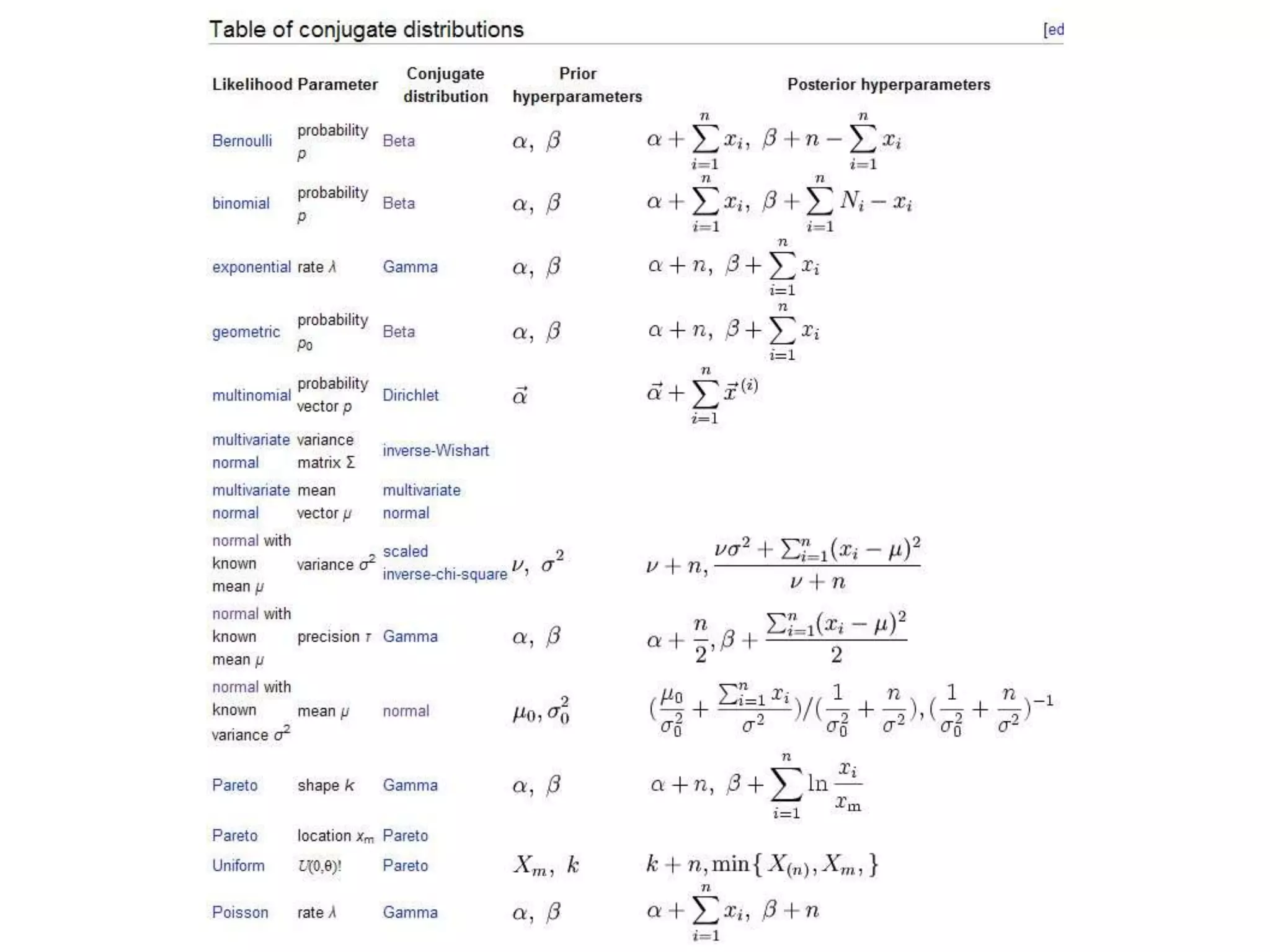
Describes Bayesian inference, modeling, and learning from observed data.
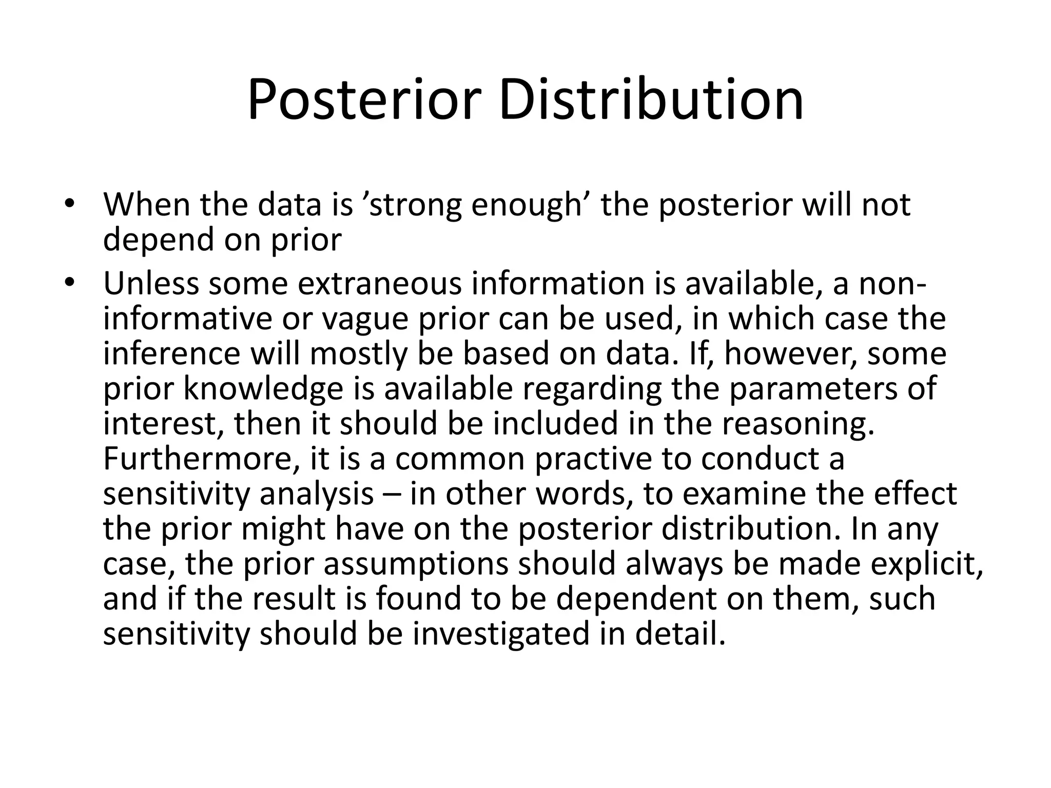
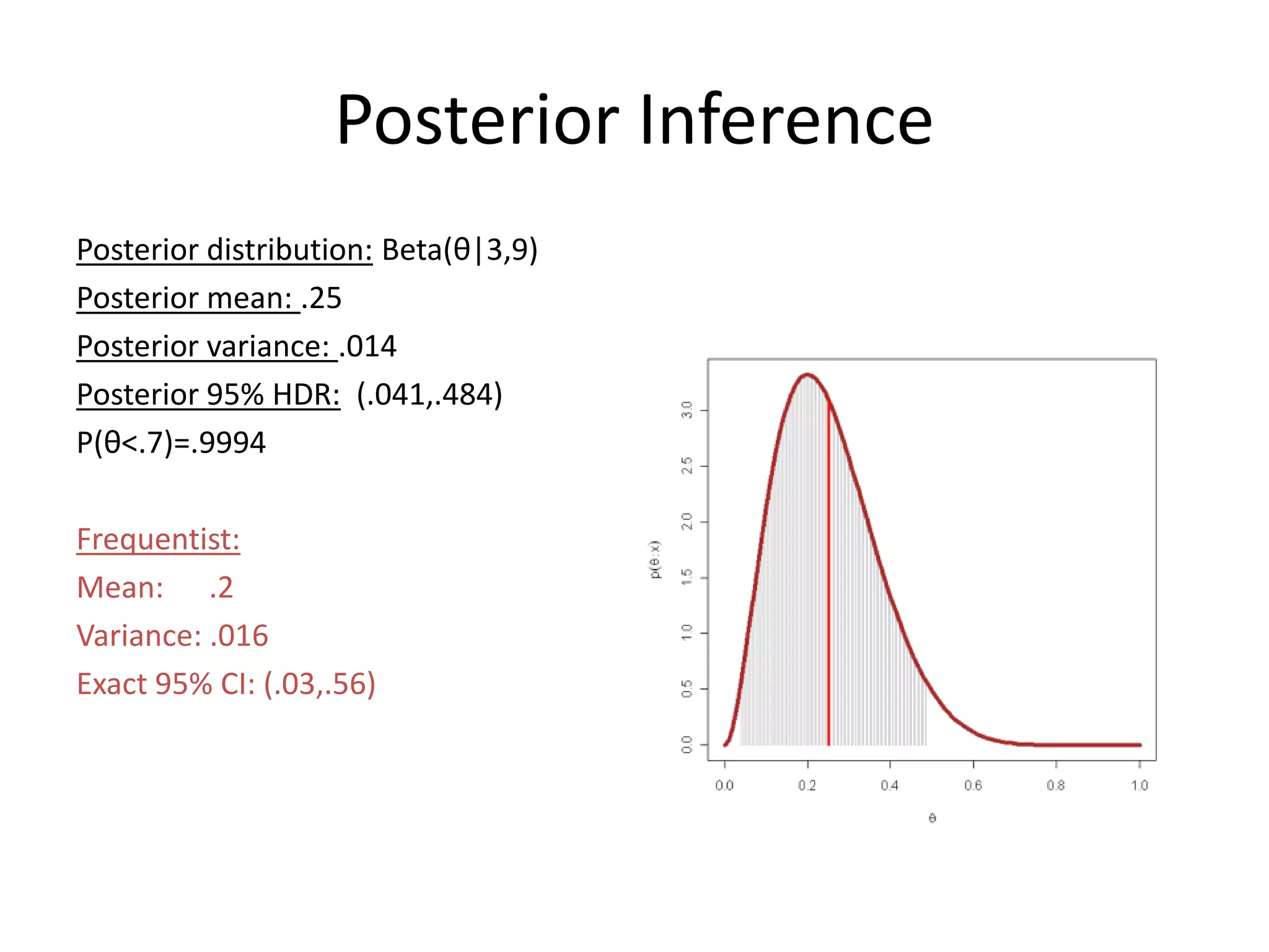
Explains how posterior distributions are formed, including computations and implications.
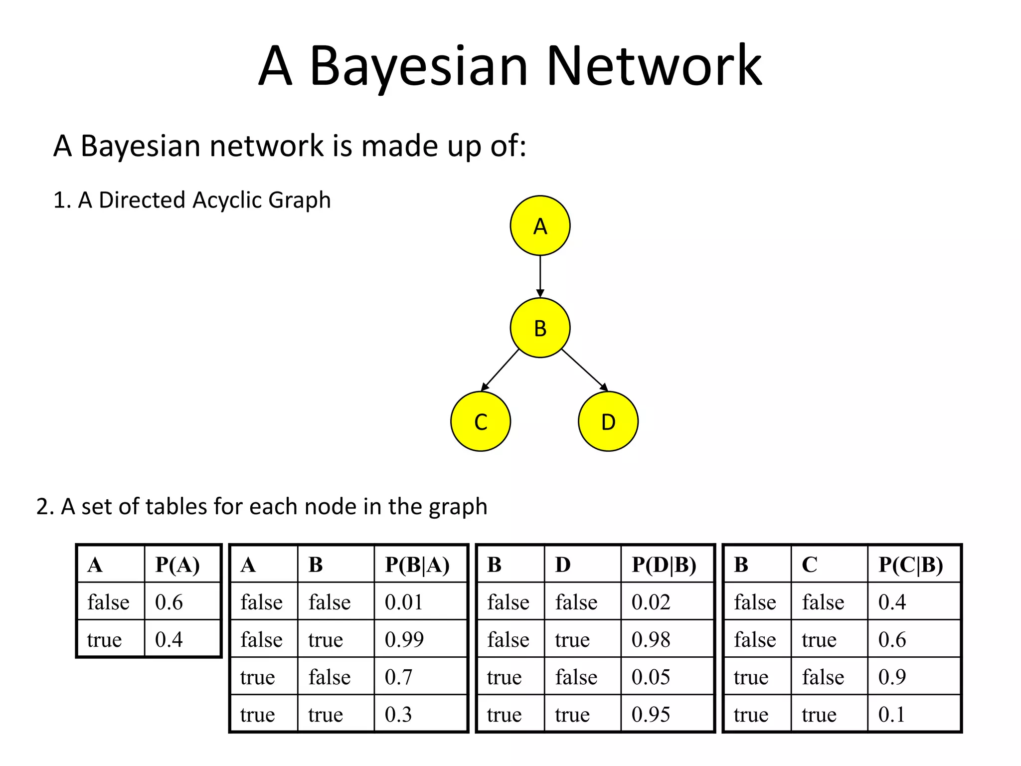
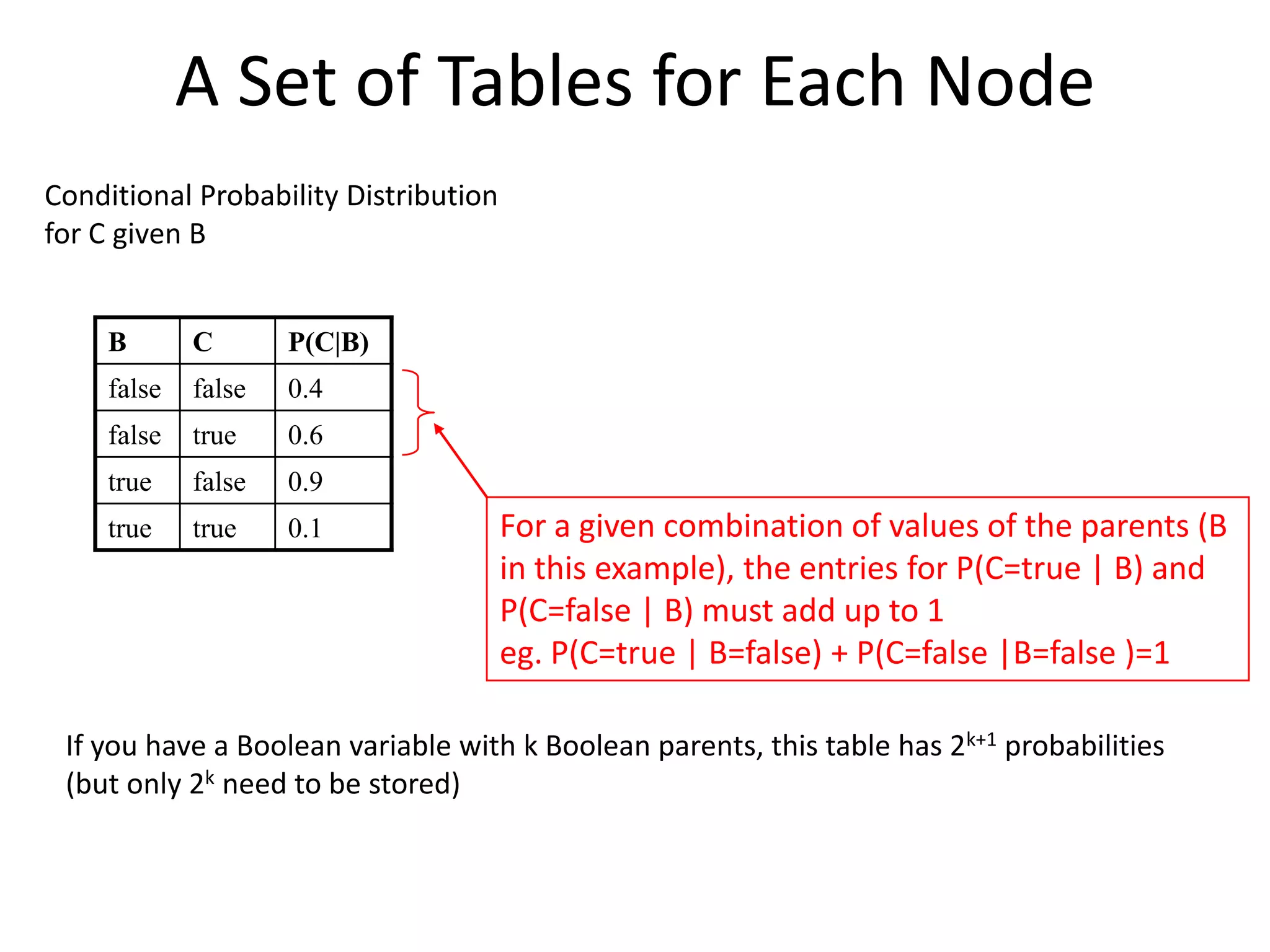
Definition and structure of Bayesian networks, including their properties.
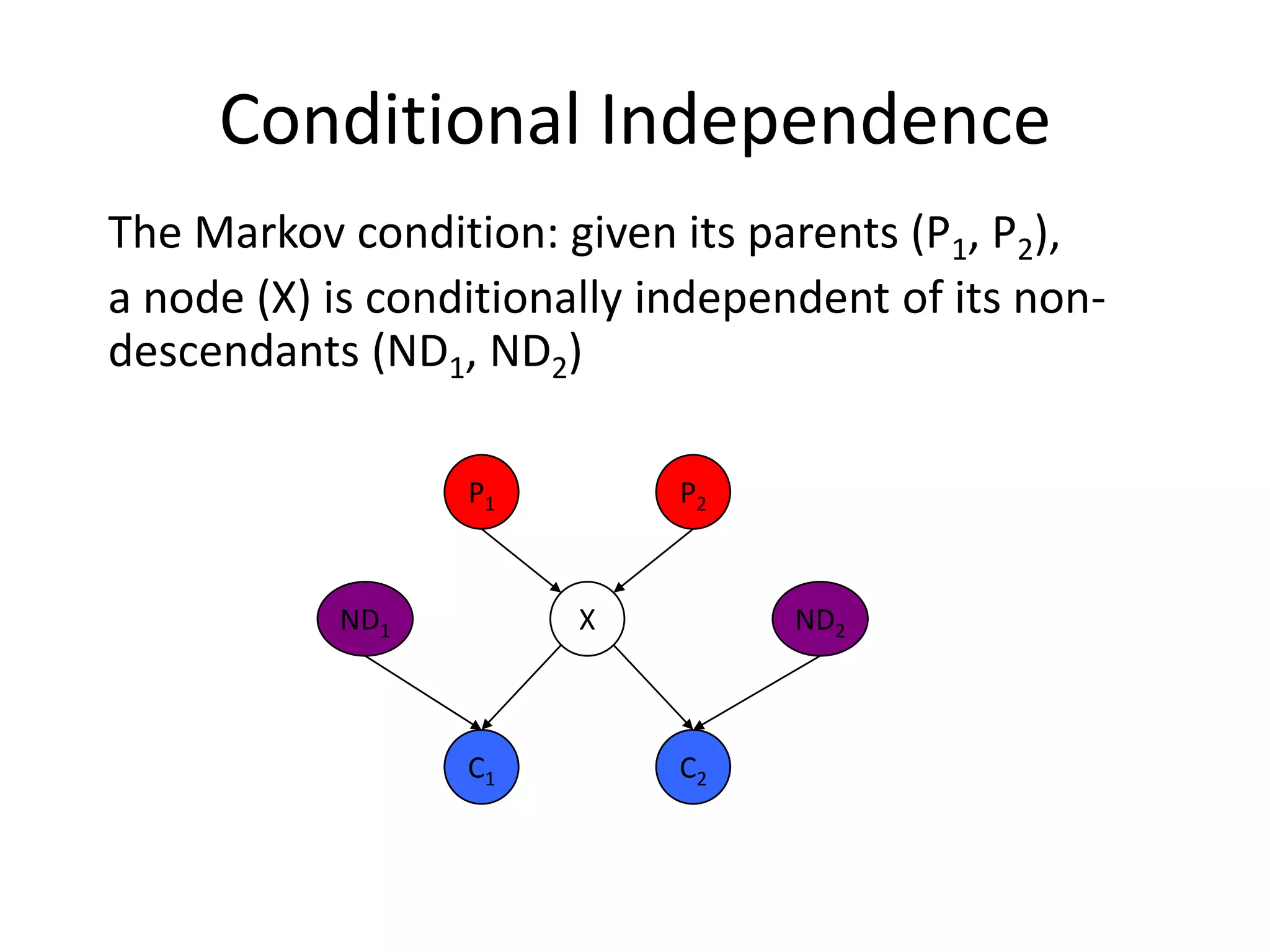
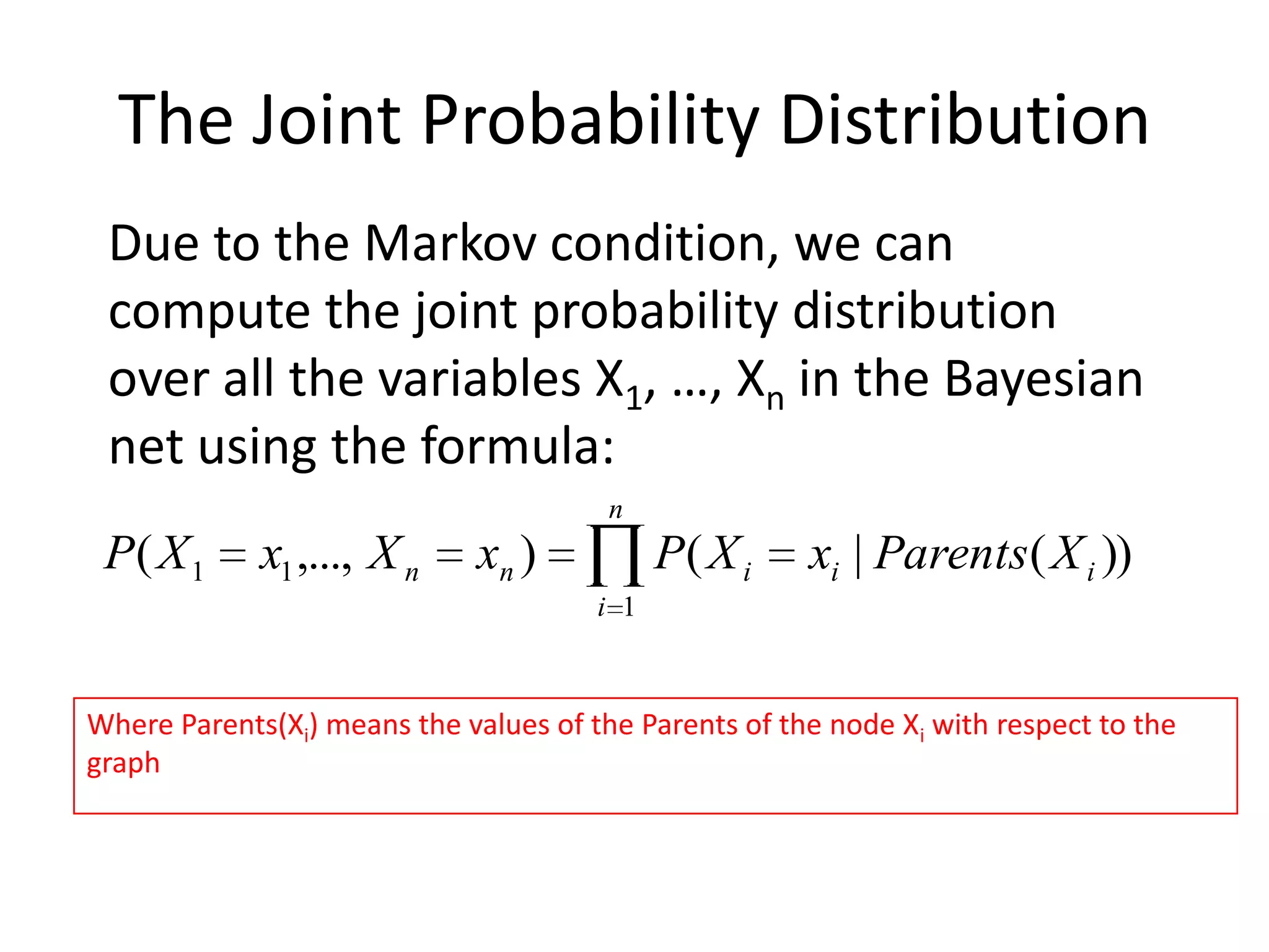
Markov condition in Bayesian networks, allowing for joint probability calculations.
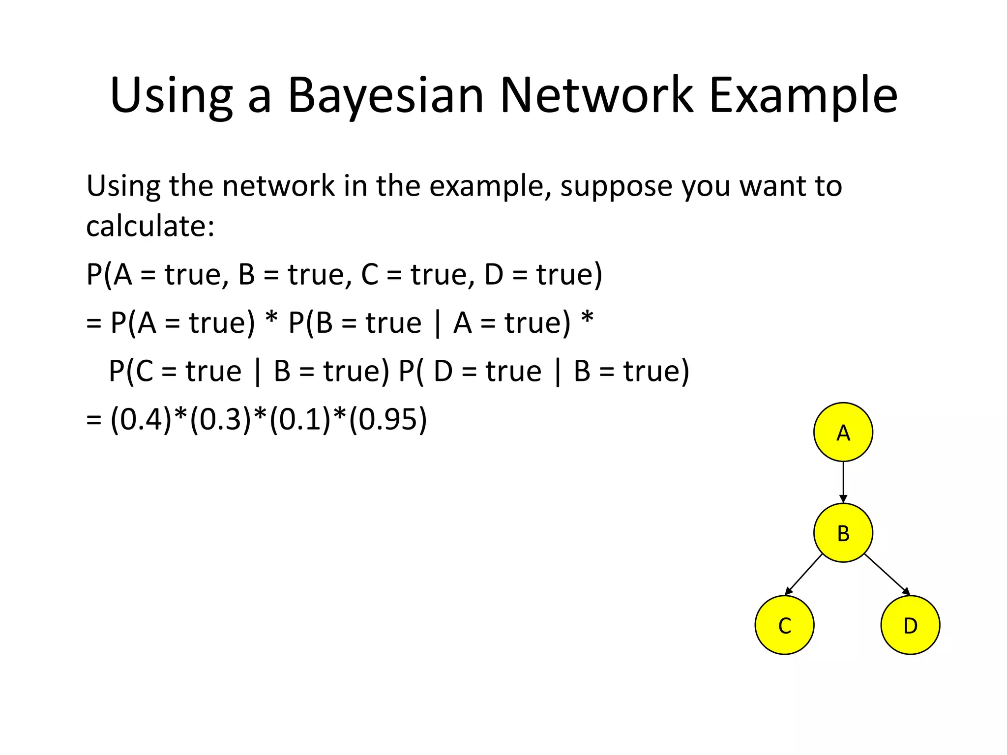
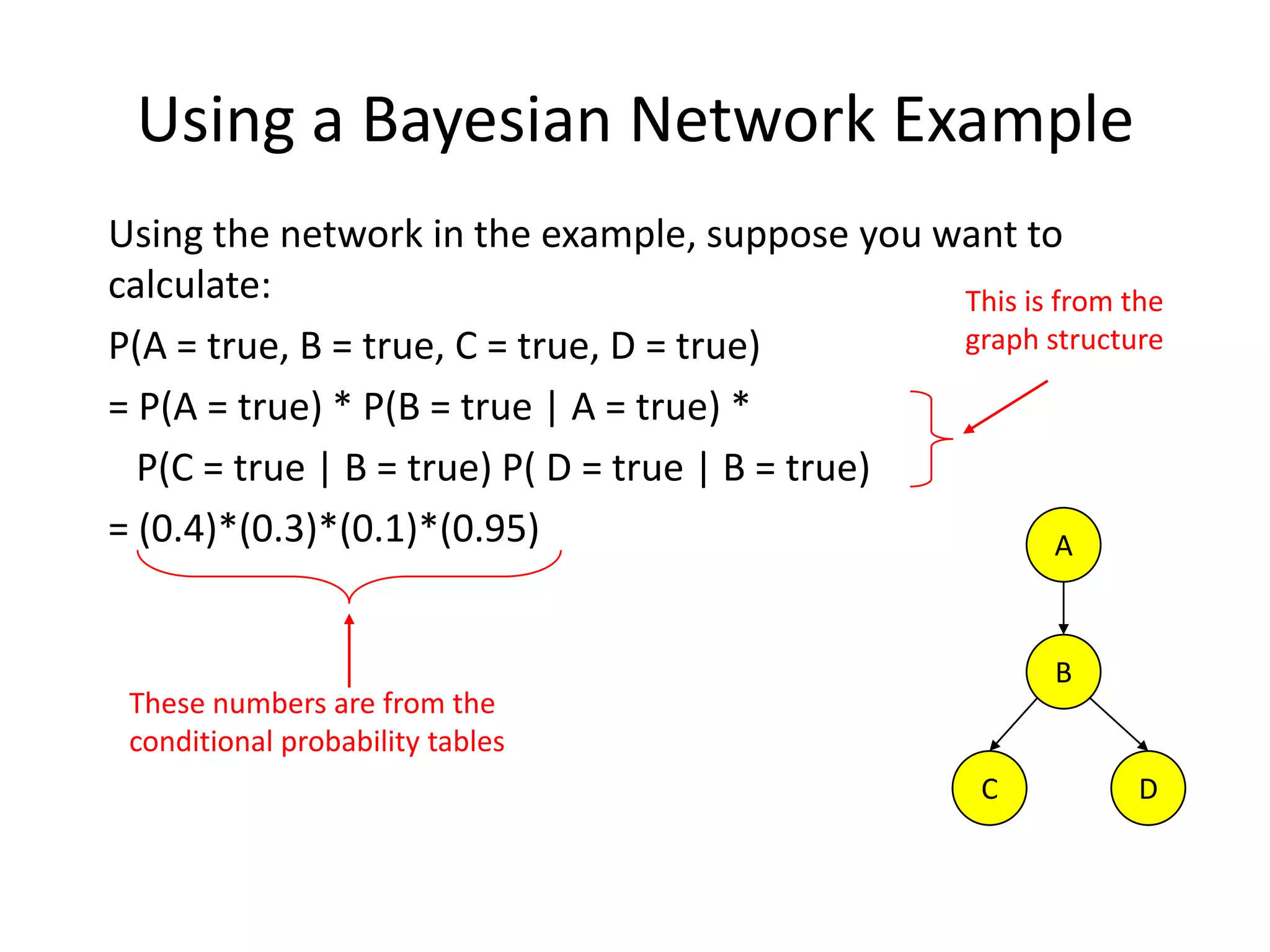
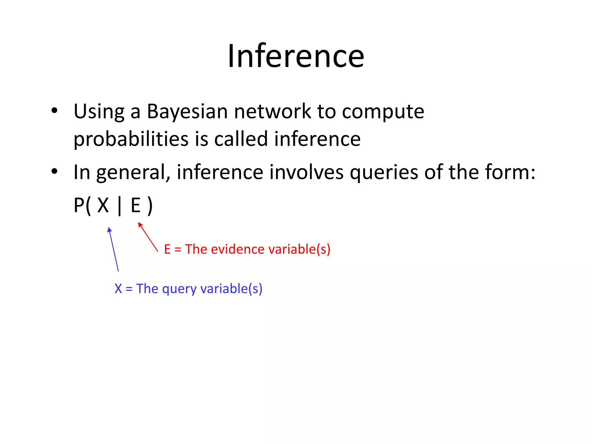
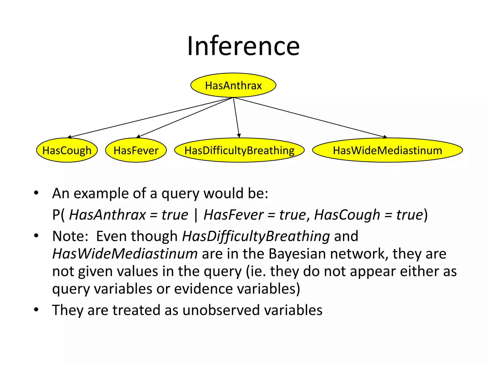
Practical example of calculating probabilities in Bayesian networks and conducting inference.