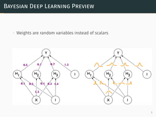
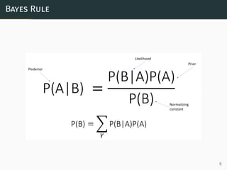
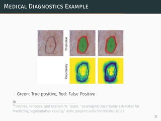
The document discusses Bayesian deep learning, emphasizing the idea that weights are treated as random variables rather than fixed scalars. It covers concepts such as maximum likelihood estimation (MLE), maximum a posteriori estimation (MAP), and various probabilistic methods like Monte Carlo sampling and variational inference for modeling uncertainty. Additionally, it addresses applications of Bayesian deep learning in critical fields such as autonomous driving and medical diagnostics, highlighting the importance of quantifying uncertainty.

1. bayesian deep learning
김규래
January 18, 2019
Sogang University SPS Lab.

2. Bayesian Deep Learning Preview
∙ Weights are random variables instead of scalars
1

3. Classic Deep Learning
∙ A classification model is expressed as f(x) = p(y ∈ c|x, θ)
”The probability that y belongs to the class c predicted from the
observation x”
∙ Training a model is defined as θ∗
= arg minθ
1
N
∑N
i L(xi, yi, θ)
”Finding the parameter θ∗
that minimizes the loss metric L”
2

4. Likelihood
A dataset is denoted as {(x, y)} = D
L(D, θ) = − log p(D|θ)
∙ How likely is the distribution p to fit the data.
∙ minimizing L is maximum likelihood estimation (MLE)
∙ The log negative probability density function (PDF) of p is often
used as MLE
∙ binary cross entropy (BCE) loss
∙ Ordinary Least Squares (OLS) loss
3

5. Maximum Likelihood Estimation
1
1https://blogs.sas.com/content/iml/2011/10/12/maximum-likelihood-estimation-in-
sasiml.html 4

6. Maximum Likelihood Estimation
For fitting a gaussian distribution to the data,
minimize L(x, y, θ)θ
= −logp(x, y | θ, σ)
= −log(
1
√
2πσ
exp −
(f(x, θ) − y)2
2σ2
)
= −log(
1
√
2πσ
) −
1
2σ2
(f(x, θ) − y)2
∝ −(f(x, θ) − y)2
L(X, Y, θ) = || f(X, θ) − Y ||2
2
5

7. Bayes Rule
6

8. Regularized Log Likelihood
L(D, θ) = −(log p(D|θ) + logp(θ))
∙ The use of Bayes’ rule to incorporate ’prior knowledge’ into the
problem
∙ Also called maximum a posteriori estimation (MAP)
p(θ|D) =
p(D|θ)p(θ)
p(D)
∝ p(D|θ)p(θ)
L(x, y, θ) = − log p(θ|D)
∝ − log (p(D|θ)p(θ))
= −(log p(D|θ) + logp(θ))
7

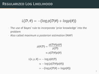
9. MAP and MLE Estimation
θ∗
MAP = arg min
θ
[− log p(D|θ) − logp(θ)]
θ∗
MLE = arg min
θ
[− log p(D|θ)]
∙ MLE and MAP estimation only estimate a fixed θ
∙ The resulting predictions are a fixed probability value
∙ In reality, θ might be better expressed as a ’distribution’
f(x) = p(y|xθ∗
MAP) ∈ R
8

10. Bayesian Inference
Eθ[ p(y|x, D) ] =
∫
p(y|x, D, θ)p(θ|D)dθ
∙ Integrating across all probable values of θ (Marginalization)
∙ Solving the integral treats θ as a distribution
∙ For a typical modern deep learning network, θ ∈ R1000000...
∙ Integrating for all possible values of θ is intractable (impossible)
9

11. Bayesian Methods
Instead of directly solving the integral,
p(y|x, D) =
∫
p(y|x, D, θ)p(θ|D)dθ
we approximate the integral and compute
∙ The expectation E[ p(y|x, D) ]
∙ The variance V[ p(y|x, D) ]
using...
∙ Monte Carlo Sampling
∙ Variational Inference (VI)
10

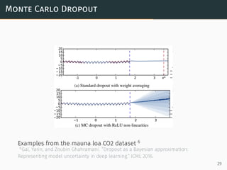
12. Output Distribution
Predicted distribution of p(y|x, D) can be visualized as
∙ Grey region is the confidence interval computed from V[ p(y|x, D) ]
∙ Blue line is the mean of the prediction E[ p(y|x, D) ]
11

13. Why Bayesian Inference?
Modelling uncertainty is becoming important in failure critical
domains
∙ Autonomous driving
∙ Medical diagnostics
∙ Algorithmic stock trading
∙ Public security
12

14. Decision Boundary and Misprediction
∙ MLE and MAP estimations lead to a fixed decision boundary
∙ ’Distant samples’ are often mispredicted with very high confidence
∙ Learning a ’distribution’ can fix this problem
13

15. Adversarial Attacks
∙ Changing even a single pixel can lead to misprediction
∙ These mispredictions have a very high confidence
2
2Su, Jiawei, Danilo Vasconcellos Vargas, and Sakurai Kouichi. ”One pixel attack for
fooling deep neural networks.” arXiv preprint arXiv:1710.08864 (2017).
14

16. Autonomous Driving
3
3Kendall, Alex, and Yarin Gal. ”What uncertainties do we need in bayesian deep
learning for computer vision?.” Advances in neural information processing systems.
2017. 15

17. Monte Carlo Intergration
p(y|x, D) =
∫
p(y|x, D, θ)p(θ|D)dθ
≈
1
S
S∑
s=0
p(y|x, D, θs)
where θs are samples from p(θ|D)
∙ Samples are directly pulled from p(θ|D)
∙ In case sampling from p is not possible, use MCMC
16

18. Monte Carlo Integration
17

19. Variational Inference
∙ Variational Inference converts an inference problem into an
optimization problem.
∙ instead of using a complicated distribution such as p(θ | D) we
find a tractable approximation q(θ, λ) parameterized with λ
∙ This is equivalent to minimizing the KL divergence of p and q
∙ Using a distribution q very different to p leads to bad solutions
minimize
λ
KL(q(x; λ) || p(x))
18

20. Variational Inference
KL(q(θ; λ)||p(θ|D))
= −
∫
q(θ; λ) log
p(θ|D)
q(θ; λ)
dθ
= −
∫
q(θ; λ) log p(θ|D)dθ +
∫
q(θ; λ) log q(θ; λ)dθ
= −
∫
q(θ; λ) log
p(θ, D)
p(D)
dθ +
∫
q(θ; λ) log q(θ; λ)dθ
= −
∫
q(θ; λ) log p(θ, D)dθ +
∫
q(θ; λ) log p(D)dθ +
∫
q(θ; λ) log q(θ; λ)dθ
= Eq[− log p(θ, D) + log q(θ; λ)] + log p(D)
where p(D) =
∫
p(θ|D)p(θ)dθ
19

21. Evidence Lower Bound (ELBO)
Because of the evidence term p(D) is intractable, optimizing the KL
divergence directly is hard.
However By reformulating the problem,
KL(q(θ; λ)||p(θ|D)) = Eq[− log p(θ, D) + log q(θ; p)] + log p(D)
log p(D) = KL(q(θ; λ)||p(θ|D)) − Eq[− log p(θ, D) + log q(θ; λ)]
log p(D) ≥ Eq[log p(θ, D) − log q(θ; λ)]
∵ KL(q(θ, λ)||p(θ|D)) ≥ 0
20

22. Evidence Lower Bound (ELBO)
maximizeλ L[q(θ; λ)] = Eq[log p(θ, D) − log q(θ; λ)]
∙ Maximizing the evidence lower bound is equivalent of minimizing
the KL divergence
∙ ELBO and KL divergence become equal at the optimum
21

23. Variational Inference
varitional inference (VI) and monte carlo methods, or even
combining both can yield very powerful solutions
22

24. Dropout Regularization
∙ Very popular deep learning regularization method before batch
normalization (9000 citations!)
∙ Make weight Wij = 0 following a Bernoulli(p) distribution
4
4Srivastava, Nitish, et al. ”Dropout: a simple way to prevent neural networks from
overfitting.” The Journal of Machine Learning Research 15.1 (2014): 1929-1958. 23

25. Dropout Regularization
∙ Regularization effect, less prone to over fitting
∙ Distribution of weight is much sparser. Good for network
compression. 24

26. Dropout As Variational Approximation
Solving MLE or MAP using dropout is variational inference.
Yarin Gal, PhD Thesis, 2016
The distribution of the weights p(W|D) is approximated using q(p, W)
q(p) is the distribution of the weight W with dropout applied
yi = (Wiyi−1 + bi) ri where ri ∼ Bern(p)
Since L2 loss and L2 regularization assumes W ∼ N(µ, σ2
), the
resulting distribution q is,
q(Wij; p) ∼ p N(µij, σ2
ij) + (1 − p) N(0, σ2
ij)
25

27. Dropout As Variational Approximation
Since the ELBO is given as,
maximizeW,p L[q(W; p)]
= Eq[ log p(W, D) − log q(W; p) ]
∝ Eq[ log p(W|D) −
p
2
|| W ||2
2 ]
=
1
N
N∑
i∈D
log p(W|xi, yi) −
p
2σ2
|| W ||2
2
is the optimization objective.
∙ if p approaches 1 or 0, q(W; p) becomes a constant distribution.
26

28. Monte Carlo Inference
Eθ[ p(y|x, D)] =
∫
p(y|x, D, θ)p(θ)dθ
≈
∫
p(y|x, D, θ)q(θ; p)dθ
= Eq[p(y|x, D)]
≈
1
T
T∑
t
p(y|x, D, θt) θt ∼ q(θ; p)
∙ Prediction is done with dropout turned on and averaging multiple
evaluations.
∙ This is equivalent to monte carlo integration by sampling from the
variational distribution.
27

29. Monte Carlo Inference
Vθ[ p(y|x, D)] ≈
1
S
S∑
s
( p(y|x, D, θs) − Eθ[p(y|x, D)] )2
Uncertainty is the variance of the samples taken from the variational
distribution.
28

30. Monte Carlo Dropout
Examples from the mauna loa CO2 dataset 6
6Gal, Yarin, and Zoubin Ghahramani. ”Dropout as a Bayesian approximation:
Representing model uncertainty in deep learning.” ICML 2016.
29

31. Monte Carlo Dropout Example
Prediction using only 10 samples 7
7Gal, Yarin, and Zoubin Ghahramani. ”Dropout as a Bayesian approximation:
Representing model uncertainty in deep learning.” ICML 2016.
30

32. Monte Carlo Dropout Example
Semantic class segmentation 8
8Kendall, Alex, and Yarin Gal. ”What uncertainties do we need in bayesian deep
learning for computer vision?.” NIPS 2017.
31

33. Monte Carlo Dropout Example
Spatial depth regression 9
9Kendall, Alex, and Yarin Gal. ”What uncertainties do we need in bayesian deep
learning for computer vision?.” NIPS 2017.
32

34. Medical Diagnostics Example
∙ Green: True positive, Red: False Positive
10
10DeVries, Terrance, and Graham W. Taylor. ”Leveraging Uncertainty Estimates for
Predicting Segmentation Quality.” arXiv preprint arXiv:1807.00502 (2018).
33

35. Medical Diagnostics Example
11
∙ Green: True positive, Blue: False Negative
11DeVries, Terrance, and Graham W. Taylor. ”Leveraging Uncertainty Estimates for
Predicting Segmentation Quality.” arXiv:1807.00502 (2018).
34

36. Possible Medical Applications
∙ Statistically correct uncertainty quantification
∙ Bandit setting clinical treatment planning (reinforcement learning)
35

37. Possible Applications: Bandit Setting
Maximizing outcome from multiple slot machines
with estimated distribution.
36

38. Possible Applications: Bandit Setting
Highest predicted outcome? or Lowest prediction uncertainty?
Choose highest predicted outcome? or explore more samples?
(Exploitation-exploration tradeoff)
37

39. Mice Skin Tumor Treatment
Mice with induced cancer tumors.
Treatment options:
∙ No threatment
∙ 5-FU (100mg/kg)
∙ imiquimod (8mg/kg)
∙ combination of imiquimod and 5-FU 38

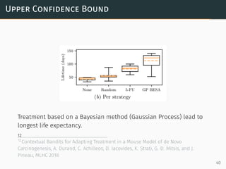
40. Upper Confidence Bound
Treatment selection policy
at = arg max
a∈A
[µa(xt) + βσ2
a(xt)]
Quality measure
R(T) =
T∑
t
[max
a∈A
µa(xt) − µa(xt)]
where A is the set of possible treatments
µ(x), σ2
(x) is the predicted mean, variance at x
39

41. Upper Confidence Bound
Treatment based on a Bayesian method (Gaussian Process) lead to
longest life expectancy.
12
12Contextual Bandits for Adapting Treatment in a Mouse Model of de Novo
Carcinogenesis, A. Durand, C. Achilleos, D. Iacovides, K. Strati, G. D. Mitsis, and J.
Pineau, MLHC 2018
40

42. References
∙ Murphy, Kevin P. ”Machine learning: a probabilistic perspective.”
(2012).
∙ Yarin Gal, ”Uncertainty in Deep Learning”, Ph.D Thesis (2016)
∙ Blundell, Charles, et al. ”Weight uncertainty in neural networks.”
arXiv preprint arXiv:1505.05424 (2015).
∙ Gal, Yarin, and Zoubin Ghahramani. ”Dropout as a Bayesian
approximation: Representing model uncertainty in deep learning.”
international conference on machine learning. 2016.
∙ Kendall, Alex, and Yarin Gal. ”What uncertainties do we need in
bayesian deep learning for computer vision?.” Advances in neural
information processing systems. 2017.
41

43. References
∙ Leibig, Christian, et al. ”Leveraging uncertainty information from
deep neural networks for disease detection.” Scientific reports 7.1
(2017): 17816.
∙ Contextual Bandits for Adapting Treatment in a Mouse Model of de
Novo Carcinogenesis A. Durand, C. Achilleos, D. Iacovides, K. Strati,
G. D. Mitsis, and J. Pineau Machine Learning for Healthcare
Conference (MLHC)
∙ Su, Jiawei, Danilo Vasconcellos Vargas, and Sakurai Kouichi. ”One
pixel attack forfooling deep neural networks.” arXiv preprint
arXiv:1710.08864 (2017).
42

44. 43