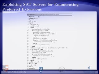
Download as PDF, PPTX
![Background
Definition
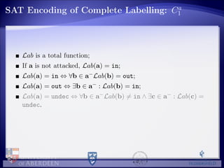
Let A, R be an argumentation framework. A total function
Lab : A → {in, out, undec} is a complete labelling iff it satisfies the
following conditions for any a ∈ A:
Lab(a) = in ⇔ ∀b ∈ a−Lab(b) = out;
Lab(a) = out ⇔ ∃b ∈ a− : Lab(b) = in;
Lab(a) = undec ⇔ ∀b ∈ a−Lab(b) = in ∧ ∃c ∈ a− : Lab(c) =
undec;
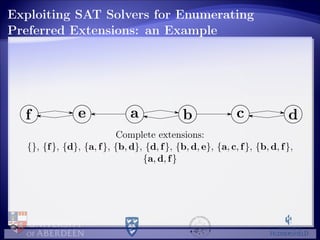
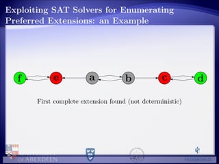
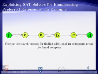
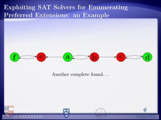
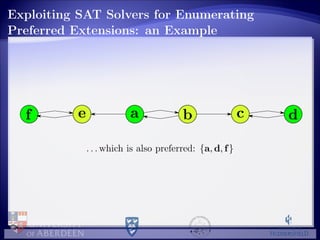
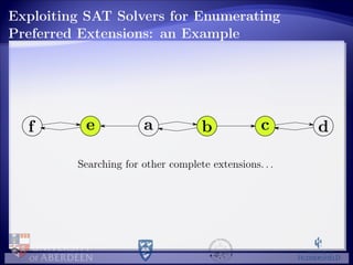
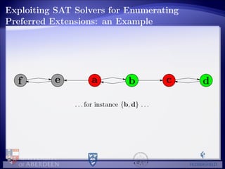
From [Caminada, 2006], preferred extensions are in one-to-one
correspondence with those complete labellings maximizing the set of
arguments labelled in.](https://image.slidesharecdn.com/cdgv-preferred-130813082908-phpapp02/85/Cerutti-TAFA2013-4-320.jpg)

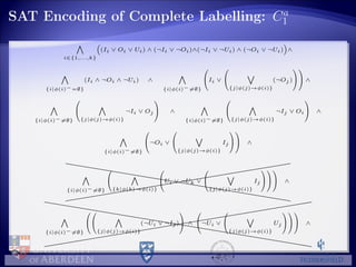


![Equivalence of the Encodings
Proposition
The encodings C1, Ca
1 , Cb
1, Cc
1, C2, C3 are equivalent.
Let us note that Ca
1 and C2 correspond to the alternative definitions
of complete labellings in [Caminada and Gabbay, 2009], where a proof
of their equivalence is provided.](https://image.slidesharecdn.com/cdgv-preferred-130813082908-phpapp02/85/Cerutti-TAFA2013-14-320.jpg)
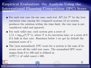
![Empirical Evaluation: the Experiment
Two SAT solvers considered (separately):
PrecoSAT [Biere, 2009], SAT Competition 2009 winner
(Application track) → PS-PRE;
Glucose
[Audemard and Simon, 2009, Audemard and Simon, 2012] SAT
Competition 2011 and SAT Challenge 2012 winner (Application
track) → PS-GLU
Random generated 2816 AFs divided in different classes according to two
dimensions:
|A|: ranging from 25 to 200 with a step of 25;
generation of the attack relations:
fixing the probability patt that there is an attack for each ordered
pair of arguments (self-attacks are included), step of 0.25
selecting randomly the number natt of attacks in it
the extreme cases of empty attack relation (patt = natt = 0) and of
fully connected attack relation (patt = 1, natt = |A|2
)](https://image.slidesharecdn.com/cdgv-preferred-130813082908-phpapp02/85/Cerutti-TAFA2013-24-320.jpg)
![Empirical Evaluation: Comparison with Aspartix,
Aspartix Meta, [Nofal et al., 2012]
60
65
70
75
80
85
90
95
100
50 100 150 200
%ofsuccess
Number of arguments
Percentage of success
ASP
ASP-META
NOF
PS-PRE
PS-GLU](https://image.slidesharecdn.com/cdgv-preferred-130813082908-phpapp02/85/Cerutti-TAFA2013-27-320.jpg)
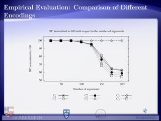
![Empirical Evaluation: Comparison with Aspartix,
Aspartix Meta, [Nofal et al., 2012]
20
30
40
50
60
70
80
90
100
50 100 150 200
IPCnormalisedto100
Number of arguments
IPC normalised to 100 with respect to the number of arguments
ASP
ASP-META
NOF
PS-PRE
PS-GLU](https://image.slidesharecdn.com/cdgv-preferred-130813082908-phpapp02/85/Cerutti-TAFA2013-28-320.jpg)
![References I
[Audemard and Simon, 2009] Audemard, G. and Simon, L. (2009).
Predicting learnt clauses quality in modern sat solvers.
In Proceedings of IJCAI 2009, pages 399–404.
[Audemard and Simon, 2012] Audemard, G. and Simon, L. (2012).
Glucose 2.1.
http://www.lri.fr/~simon/?page=glucose.
[Biere, 2009] Biere, A. (2009).
P{re,ic}osat@sc’09.
In SAT Competition 2009.
[Caminada, 2006] Caminada, M. (2006).
On the issue of reinstatement in argumentation.
In Proceedings of JELIA 2006, pages 111–123.
[Caminada and Gabbay, 2009] Caminada, M. and Gabbay, D. M. (2009).
A logical account of formal argumentation.
Studia Logica (Special issue: new ideas in argumentation theory), 93(2–3):109–145.
[Nofal et al., 2012] Nofal, S., Dunne, P. E., and Atkinson, K. (2012).
On preferred extension enumeration in abstract argumentation.
In Proceedings of COMMA 2012, pages 205–216.](https://image.slidesharecdn.com/cdgv-preferred-130813082908-phpapp02/85/Cerutti-TAFA2013-30-320.jpg)

The document presents a SAT-based approach for computing preferred extensions in abstract argumentation, detailing the theoretical framework, algorithm, and empirical evaluation. It explores complete labellings, their encodings, and how to use SAT solvers for enumerating preferred extensions, citing performance metrics and comparisons with existing systems. The authors conclude that their method demonstrates superior performance and outline future work on broader argumentation semantics.