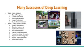
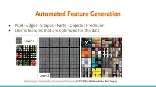
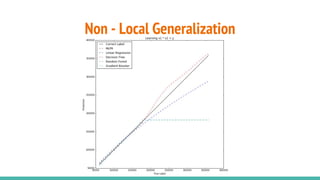
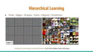
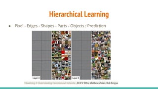
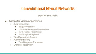
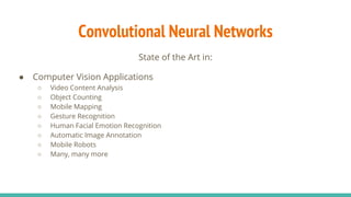
The document provides a comprehensive overview of convolutional neural networks (CNNs), detailing their structure, functionality, and applications in various fields such as computer vision and natural language processing. It discusses key concepts including automated feature engineering, non-local generalization, model optimization, and the advantages of deep learning over traditional algorithms. Additionally, it highlights CNN's state-of-the-art performance in tasks like object recognition, speech recognition, and image segmentation.

1. Understanding Convolutional Neural Networks
Jeremy Nixon

2. Jeremy Nixon
● Machine Learning Engineer at the Spark Technology Center
● Contributor to MLlib, dedicated to scalable deep learning
○ Author of Deep Neural Network Regression
● Previously, Applied Mathematics to Computer Science & Economics at
Harvard

3. Structure
1. Introduction / About
2. Motivation
a. Comparison with major machine learning algorithms
b. Tasks achieving State of the Art
c. Applications / Specific Concrete Use Cases
3. The Model / Forward Pass
4. Framing Deep Learning
a. Automated Feature Engineering
b. Non-local generalization
c. Compositionality
i. Hierarchical Learning
ii. Exponentially Model Flexibility
d. Learning Representation
i. Transformation for Linear Separability
ii. Input Space Contortion
e. Extreme flexibility allowing benefits to large datasets
5. Optimization / Backward Pass
6. Conclusion

4. Many Successes of Deep Learning
1. CNNs - State of the art
a. Object Recognition
b. Object Localization
c. Image Segmentation
d. Image Restoration
e. Music Recommendation
2. RNNs (LSTM) - State of the Art
a. Speech Recognition
b. Question Answering
c. Machine Translation
d. Text Summarization
e. Named Entity Recognition
f. Natural Language Generation
g. Word Sense Disambiguation
h. Image / Video Captioning
i. Sentiment Analysis

5. Ever trained a Linear Regression Model?

6. Linear Regression Models
Major Downsides:
Cannot discover non-linear structure in data.
Manual feature engineering by the Data Scientist. This is time consuming and
can be infeasible for high dimensional data.

7. Decision Tree Based Model? (RF, GB)

8. Decision Tree Models
Upside:
Capable of automatically picking up on non-linear structure.
Downsides:
Incapable of generalizing outside of the range of the input data.
Restricted to cut points for relationships.
Thankfully, there’s an algorithmic solution.

9. Neural Networks
Properties
1. Non-local generalization
2. Learning Non-linear structure
3. Automated feature generation

10. Generalization Outside Data Range

11. Feedforward Neural Network
X = Normalized Data, W1
, W2
= Weights, b = Bias
Forward:
1. Multiply data by first layer weights | (X*W1
+ b1
)
2. Put output through non-linear activation | max(0, X*W1
+ b1
)
3. Multiply output by second layer weights | max(0, X*W1
+ b) * W2
+ b2
4. Return predicted outputs

12. The Model / Forward Pass
● Forward
○ Convolutional layer
■ Procedure + Implementation
■ Parameter sharing
■ Sparse interactions
■ Priors & Assumptions
○ Nonlinearity
■ Relu
■ Tanh
○ Pooling Layer
■ Procedure + Implementation
■ Extremely strong prior on image, invariance to small translation.
○ Fully Connected + Output Layer
○ Putting it All Together

13. Convolutional Layer
Input Components:
1. Input Image / Feature Map
2. Convolutional Filter / Kernel / Parameters / Weights
Output Component:
1. Computed Output Image / Feature Map

14. Convolutional Layer
Goodfellow, Bengio, Courville

15. Convolutional Layer
Leow Wee Kheng

16. Convolutional Layer

17. 1. Every filter weight is used over the entire input.
a. This differs strongly from a fully connected network where each weight corresponds to a
single feature.
2. Rather than learning a separate set of parameters for each location, we
learn a single set.
3. Dramatically reduces the number of parameters we need to store.
Parameter Sharing

18. Bold Assumptions
1. Convolution be thought of as a fully connected layer with an infinitely strong prior probability that
a. The weights for one hidden unit must be identical to the weights of its neighbor. (Parameter
Sharing)
b. Weights must be zero except for in a small receptive field (Sparse Interactions)
2. Prior assumption of invariance to locality
a. Assumptions overcome data augmentation with translational shifts
i. Other useful transformations include rotations, flips, color perturbations, etc.
b. Equivariant to translation as a result of parameter sharing, but not to rotation or scale (closer
in / farther)

19. Sparse Interactions
Strong prior on the
locality of information.
Deep networks end up
with greater connectivity.

20. Non-Linearities
● Element-wise transformation (Applied individually over every element)
Relu Tanh

21. Max Pooling
Downsampling.
Takes the max value
of regions of the input
image or filter map.
Imposes extremely
strong prior of
invariance to
translation.

22. Mean Pooling

23. Output Layer
● Output for classification is often a Softmax function + Cross Entropy loss.
● Output for regression is a single output from a linear (identity) layer with a
Sum of Squared Error loss.
● Feature map can be flattened into a vector to transition to a fully
connected layer / softmax.

24. Putting it All Together
We can construct architectures that combine
convolution, pooling, and fully connected layers
similar to the examples given here.

25. Framing Deep Learning
1. Automated Feature Engineering
2. Non-local generalization
3. Compositionality
a. Hierarchical Learning
b. Exponential Model Flexibility
4. Extreme flexibility opens up benefits to large datasets
5. Learning Representation
a. Input Space Contortion
b. Transformation for Linear Separability

26. Automated Feature Generation
● Pixel - Edges - Shapes - Parts - Objects : Prediction
● Learns features that are optimized for the data

27. Non - Local Generalization

28. Hierarchical Learning
● Pixel - Edges - Shapes - Parts - Objects : Prediction

29. Hierarchical Learning
● Pixel - Edges - Shapes - Parts - Objects : Prediction

30. Exponential Model Flexibility
● Deep Learning assumes data was generated by a composition of factors
or features.
○ DL has been most successful when this assumption holds.
● Exponential gain in the number of relationships that can be efficiently
models through composition.

31. Model Flexibility and Dataset Size
Large datasets allow the fitting of
extremely wide & deep models, which
would have overfit in the past.
A combination of large datasets, large &
flexible models, and regularization
techniques (dropout, early stopping, weight
decay) are responsible for success.

32. Learning Representation:
Transform for Linear Separability
Hidden Layer
+
Nonlinearity
Chris Olah:
http://colah.github.io/posts/2014-03-NN-Manifolds-Topology/

33. The goal:
Iteratively improve the filter weights so that they generate correct predictions.
We receive an error signal from the difference between our predictions and
the true outcome.
Our weights are adjusted to reduce that difference.
The process of computing the correct adjustment to our weights at each layer
is called backpropagation.
Backward Pass / Optimization

34. Convolutional Neural Networks
State of the Art in:
● Computer Vision Applications
○ Autonomous Cars
■ Navigation System
■ Pedestrian Detection / Localization
■ Car Detection / Localization
■ Traffic Sign Recognition
○ Facial Recognition Systems
○ Augmented Reality
■ Visual Language Translation
○ Character Recognition

35. Convolutional Neural Networks
State of the Art in:
● Computer Vision Applications
○ Video Content Analysis
○ Object Counting
○ Mobile Mapping
○ Gesture Recognition
○ Human Facial Emotion Recognition
○ Automatic Image Annotation
○ Mobile Robots
○ Many, many more

36. References
● CS 231: http://cs231n.github.io/
● Goodfellow, Bengio, Courville: http://www.deeplearningbook.org/
● Detection as DNN Regression: http://papers.nips.cc/paper/5207-deep-neural-networks-for-object-detection.pdf
● Object Localization: http://arxiv.org/pdf/1312.6229v4.pdf
● Pose Regression: https://www.robots.ox.ac.uk/~vgg/publications/2014/Pfister14a/pfister14a.pdf
● Yuhao Yang CNN: (https://issues.apache.org/jira/browse/SPARK-9273)
● Neural Network Image: http://cs231n.github.io/assets/nn1/neural_net.jpeg
● Zeiler / Fergus: https://arxiv.org/pdf/1311.2901v3.pdf