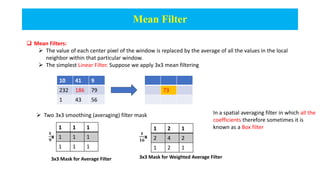
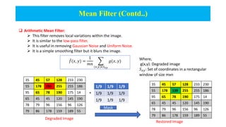
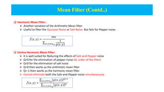
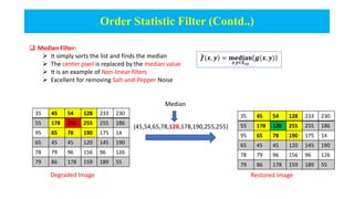
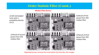
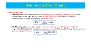
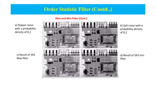
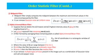
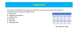
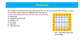
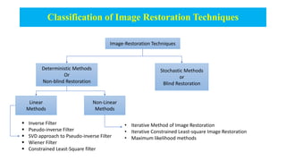
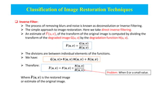
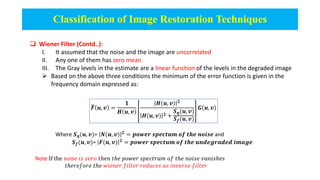
Image Restoration in the Presence of Noise only
 Image Denoising:
 The goal of denoising is to remove the noise while retaining as much as possible the important signal
features.
 Denoising can be done through filtering, which can be either linear filtering or non-linear filtering.
 Spatial Filter, which is used in image smoothing or sharpening and also used for removing noise.
Image Restoration Spatial Filters
Mean Filters Order Statistic Filters
Contra-harmonic Mean
Arithmetic Mean Filter
Geometric Mean Filter
Harmonic Mean Filter
Alpha Trimmed Filter
Median Filter
Max and Min filter
Mid point Filter
Mean Filter
 Mean Filters:
 The value of each center pixel of the window is replaced by the average of all the values in the local
neighbor within that particular window.
 The simplest Linear Filter. Suppose we apply 3x3 mean filtering
10 41 9
232 186 79
1 43 56
73
1 1 1
1 1 1
1 1 1
𝟏
𝟗
x
1 2 1
2 4 2
1 2 1
𝟏
𝟏𝟔
x
 Two 3x3 smoothing (averaging) filter mask
3x3 Mask for Average Filter 3x3 Mask for Weighted Average Filter
In a spatial averaging filter in which all the
coefficients therefore sometimes it is
known as a Box filter
Mean Filter (Contd..)
 Arithmetic Mean Filter:
 This filter removes local variations within the image.
 It is similar to the low-pass filter.
 It is useful in removing Gaussian Noise and Uniform Noise.
 It is a simple smoothing filter but it blurs the image.
𝑓(𝑥, 𝑦) =
1
𝑚𝑛
(𝑥,𝑦)∈𝑆𝑥𝑦
𝑔(𝑥, 𝑦)
Where,
g(x,y): Degraded image
𝑆𝑥𝑦: Set of coordinates in a rectangular
window of size mxn
1/9 1/9 1/9
1/9 1/9 1/9
1/9 1/9 1/9
35 45 57 128 233 230
55 178 255 255 255 186
95 65 78 190 175 14
65 45 45 120 145 190
78 79 96 156 96 126
79 86 178 159 189 55
*
Mask
Degraded Image
35 45 57 128 233 230
55 178 139 255 255 186
95 65 78 190 175 14
65 45 45 120 145 190
78 79 96 156 96 126
79 86 178 159 189 55
Restored Image
Mean Filter (Contd..)
 Geometric Mean Filter:
 Variation of Arithmetic Mean
 Geometric mean filter achieves smoothing
comparable to the arithmetic mean filter but
tends to lose less image detail in the process.
 Retains image details better than the
arithmetic mean.
 It is ineffective for Pepper type of noise.
 Primarily used to eliminate Gaussian Noise
𝑓 𝑥, 𝑦 =
(𝑥,𝑦)∈𝑆𝑥𝑦
𝑔(𝑥, 𝑦)
1
𝑚𝑛
Fig: a) X-ray image
b) Gaussian noise image
c) Arithmetic mean
d) Geometric mean
Mean Filter (Contd..)
 Harmonic Mean Filter:
 Another variation of the Arithmetic Mean filter.
 Useful to filter the Gaussian Noise or Salt Noise. But fails for Pepper noise.
𝑓(𝑥, 𝑦) =
𝑚𝑛
(𝑥,𝑦)∈𝑆𝑥𝑦
1
𝑔(𝑥, 𝑦)
 Contra-Harmonic Mean Filter:
 It is well suited for Reducing the effects of Salt-and-Pepper noise
 Q>0 for the elimination of pepper noise (Q: order of the filter)
 Q<0 for the elimination of salt noise
 Q=0 then works as the arithmetic mean filter
 Q=-1 then works as the harmonic mean filter
 Cannot eliminate both the Salt-and-Pepper noise simultaneously.
𝑓(𝑥, 𝑦) =
(𝑥,𝑦)∈𝑆𝑥𝑦
𝑔(𝑥, 𝑦) 𝑄+1
(𝑥,𝑦)∈𝑆𝑥𝑦
𝑔(𝑥, 𝑦) 𝑄
Mean Filter (Contd..)
a)Image
corrupted
by Pepper
Noise with
the
probability
of 0.1
c) 3X3
Contra-
harmoni
c filter of
order
Q=1.5
b)Image
corrupted
by Salt
Noise with
the
probability
of 0.1
d) 3X3
Contra-
harmonic
filter of
order
Q=-1.5
Mean Filter (Contd..)
Wrong sign of Contra harmonic filter
Pepper noise Salt noise
Order Statistic Filter
 Order statistic filters are also known as Rank, or Order Filters
 These filters are not based on convolution
 These filters are differentiated based on how they choose the values in the sorted list.
 The position indicates the rank.
 Operate on a neighborhood around a reference pixel by ordering (Ranking) the pixel values and then
performing an operation on those ordered values to obtain the new value for the reference pixel.
 They perform very well in the presence of Salt-and-Pepper noise but are more computationally expensive
as compared to mean filters.
Order Statistic Filter (Contd..)
 Median Filter:
 It simply sorts the list and finds the median
 The center pixel is replaced by the median value
 It is an example of Non-linear filters
 Excellent for removing Salt-and-Pepper Noise
𝒇(𝒙, 𝒚) = 𝐦𝐞𝐝𝐢𝐚𝐧
𝒙,𝒚∈𝑺𝒙𝒚
𝒈(𝒙, 𝒚)
35 45 54 128 233 230
55 178 255 255 255 186
95 65 78 190 175 14
65 45 45 120 145 190
78 79 96 156 96 126
79 86 178 159 189 55
(45,54,65,78,128,178,190,255,255)
Median
35 45 54 128 233 230
55 178 128 255 255 186
95 65 78 190 175 14
65 45 45 120 145 190
78 79 96 156 96 126
79 86 178 159 189 55
Degraded Image Restored Image
Order Statistic Filter (Contd..)
Median Filter (Cont.)
a) Salt-and-pepper
noise with a
probability density
of 0.2
b) Result of first
passes from 3X3
median filter
c) Result of second
passes from 3X3
median filter
d) Result of third
passes from 3X3
median filter
Repeated passes remove the noise better but also blur the images
Order Statistic Filter (Contd..)
 Max and Min Filter:
 Max filter: Replace the pixel value with the Maximum of the Gray level (The Brightest point) in the
neighborhood of that pixel. It is also known as 100𝑡ℎ
𝑝𝑒𝑟𝑐𝑒𝑛𝑡𝑖𝑙𝑒 filter. Used for finding the
brightest points of images and removing the Pepper noise.
𝒇(𝒙, 𝒚) = 𝐌𝐚𝐱
𝒙,𝒚∈𝑺𝒙𝒚
𝒈(𝒙, 𝒚)
𝒇(𝒙, 𝒚) = 𝐦𝐢𝐧
𝒙,𝒚∈𝑺𝒙𝒚
𝒈(𝒙, 𝒚)
 Min filter: Replace the pixel value with the minimum of the Gray level (The darkest point) in the
neighborhood of that pixel. It is also known as zeroth 𝑝𝑒𝑟𝑐𝑒𝑛𝑡𝑖𝑙𝑒 filter. Used for finding the darkest points
and removing the Salt noise.
Order Statistic Filter (Contd..)
Max and Min Filter (Cont.)
a) Pepper noise
with a probability
density of 0.2
c) Result of 3X3
Max filter
d) Result of 3X3 min
filter
b) Salt noise with a
probability density
of 0.2
Order Statistic Filter (Contd..)
 Alpha-trimmed Mean Filter:
 Suppose that we delete the d/2 lowest and d/2 highest intensity value of g(x,y) in the
neighborhood of 𝑆𝑥𝑦
 Let 𝑔𝑟(x,y) represent the remaining mn-d pixels.
 A filter formed by averaging these remaining pixels is called Alpha-trimmed Mean Filter.
 Where the value of d can range between 0 to mn-1.
 If d=0 then the filter becomes an arithmetic mean filter.
 If d=mn-1 then the filter becomes the median filter.
 It can remove multiple types of noise present in the image such as a combination of Gaussian noise
and salt-and-pepper noise
𝑺𝒙𝒚: Set of coordinates in a rectangular window of
size mxn
𝑓(𝑥, 𝑦) =
1
𝑚𝑛 − 𝑑
(𝑥,𝑦)∈𝑆𝑥𝑦
𝑔𝑟(𝑥, 𝑦)
 Midpoint Filter:
 Midpoint filter simply computes the midpoint between the maximum and minimum values in the
area encompassed by the filter.
 It can remove Gaussian noise or Uniform noise 𝒇(𝒙, 𝒚) =
𝟏
𝟐
𝐌𝐚𝐱
𝒙,𝒚∈𝑺𝒙𝒚
𝒈(𝒙, 𝒚) + 𝐦𝐢𝐧
𝒙,𝒚∈𝑺𝒙𝒚
𝒈(𝒙, 𝒚)
Numerical
Q1. Consider the following 5x5 image what will be the new value of the pixels (2,2) and (3,2), if
smoothing is done using a 3x3 neighborhood?
a) Mean filter
b) Weighted Average filter
c) Median Filter
d) Min filter
e) Max filter
f) Mid-point filter
0 1 0 2 7
2 7 7 4 0
5 6 4 3 3
1 1 0 7 5
5 4 2 2 5
Fig1: Degraded image
Numerical
Q2. Consider the following 5x5 image, What will be the new value of the pixels (0,0) and (0,2), and (1,4)
if smoothing is done using a 3x3 neighborhood? (see Fig 1.1)
(Assume zero-padding technique for pixels close to boundaries).
a) Mean filter
b) Weighted Average filter
c) Median Filter
d) Min filter
e) Max filter
f) Mid-point filter
0 0 0 0 0 0 0
0 0 1 0 2 7 0
0 2 7 7 4 0 0
0 5 6 4 3 3 0
0 1 1 0 7 5 0
0 5 4 2 2 5 0
0 0 0 0 0 0 0
Fig1.1: Degraded image with
zero-padding
Numerical
Q3. Consider the following 5x5 image What will be the new value of the pixels (0,0) and (0,2), and (1,4) if
smoothing is done using a 3x3 neighborhood? (see Fig 1.2)
(Assume wrap-around technique for pixels close to boundaries).
a) Mean filter
b) Weighted Average filter
c) Median Filter
d) Min filter
e) Max filter
f) Mid-point filter
5 5 4 2 2 5 5
7 0 1 0 2 7 0
0 2 7 7 4 0 2
3 5 6 4 3 3 5
5 1 1 0 7 5 1
5 5 4 2 2 5 5
7 0 1 0 2 7 0
Fig1.2: Degraded image with
wrap-around boundaries
Numerical
Q4. Consider the following 4x4 image as in Fig 1.3. Filter this image using a median filter with the filter
mask as given in Fig. 1.4.
(Assume replicate padding technique for pixels close to boundaries).
Fig1.2: Degraded image with
replicate-padding
3 3 2 1 4 4
3 3 2 1 4 4
5 5 2 6 3 3
7 7 9 1 4 4
2 2 4 6 8 8
2 2 4 6 8 8
Fig 1.4: Filter Mask
Classification of Image Restoration Techniques
Image-Restoration Techniques
Deterministic Methods
Or
Non-blind Restoration
Stochastic Methods
or
Blind Restoration
Linear
Methods
Non-Linear
Methods
 Inverse Filter
 Pseudo-inverse Filter
 SVD approach to Pseudo-inverse Filter
 Wiener Filter
 Constrained Least-Square filter
• Iterative Method of Image Restoration
• Iterative Constrained Least-square Image Restoration
• Maximum likelihood methods
Classification of Image Restoration Techniques
 Inverse Filter:
 The process of removing blurs and noise is known as deconvolution or Inverse Filtering.
 The simple approach to image restoration. Here we take direct inverse filtering.
 An estimate of 𝐹 𝑢, 𝑣 , of the transform of the original image is computed by dividing the
transform of the degraded image G(u, v) by the degradation function H(u, v).
 The divisions are between individual elements of the functions.
 We have:
 Therefore:
Where 𝑭 𝒖, 𝒗 is the restored image
or estimate of the original image.
𝑭 𝒖, 𝒗 =
𝑮 𝒖, 𝒗
𝑯 𝒖, 𝒗
𝑮(𝒖, 𝒗)= F(𝒖, 𝒗) H 𝒖, 𝒗 + 𝑵(𝒖, 𝒗)
𝑭 𝒖, 𝒗 = 𝑭 𝒖, 𝒗 +
𝑵 𝒖, 𝒗
𝑯 𝒖, 𝒗
Problem: When 0 or a small value.
Classification of Image Restoration Techniques
 Inverse Filtering (Contd.):
 Even if we know the degradation function H(u, v), we can not recover the degraded image
exactly because N(u, v) is a random function whose Fourier transform is not known.
 If the degradation function has zero or very small values, then the ratio
𝑵 𝒖,𝒗
𝑯 𝒖,𝒗
could easily
dominate the estimate.
 One approach to get around the zero or small-value problem is to limit the filter
frequencies to values near the origin.
 We know H(u,v) represents the spectrum of the Point-spread function(PSF). Mostly, the
PSF is a low-pass filter which implies that H(0,0) is usually the highest value of H(u, v) in
the frequency domain.
 Thus, by limiting the analysis to frequencies near the origin, we reduce the probability of
encountering zero values.
 Degradation function with k=0.0025.
𝑯 𝒖, 𝒗 = 𝒆
−𝒌 𝒖−
𝑴
𝟐
𝟐
+ 𝒗−
𝑵
𝟐
𝟐
𝟓
𝟔
The
𝑴
𝟐
𝒂𝒏𝒅
𝑵
𝟐
constants are offset values; they center the function. In this case M=N=480.
Classification of Image Restoration Techniques
Original Image
Degraded
Image with
k=0.0025
Degraded
Image with
k=0.001
Degraded
Image with
k=0.00025
Inverse Filtering (Contd.)
Classification of Image Restoration Techniques
Full Inverse
Filtering for
k=0.0025
Cutoff values of
the ratio
𝑮 𝒖,𝒗
𝑯 𝒖,𝒗
outside a radius
of 40
Inverse Filtering (Contd.)
Cutoff values of
the ratio
𝑮 𝒖,𝒗
𝑯 𝒖,𝒗
outside a radius
of 70
Cutoff values of
the ratio
𝑮 𝒖,𝒗
𝑯 𝒖,𝒗
outside a radius
of 85
Classification of Image Restoration Techniques
 Pseudo-Inverse Filtering:
 To avoid the problem of inverse filtering, another solution is to design a Transfer function
called a pseudo-inverse filter defined as:
𝟏
𝑯 𝒖,𝒗
=
𝟏
𝑯 𝒖,𝒗
, 𝑖𝑓 𝑯 𝒖, 𝒗 > 𝜖, otherwise 𝜖 𝑖𝑓 𝑯 𝒖, 𝒗 ≤ 𝜖
 Where 𝝐 is Threshold value that affects the restored image. With no clear objective
selection of 𝝐, restored images generally noisy and not suitable for further analysis
 Major Drawback of Inverse Filter: It is not perform well in the presence of noise. So better
to use Wiener Filter.
Classification of Image Restoration Techniques
 Wiener Filter:
 It is also known as a minimum Mean Square Error Filter or Least Square Error Filter
 This approach incorporates both the degradation function and statistical characteristics of
noise into the restoration process.
 The objective is to find an estimate of the uncorrupted image such that the mean square
error between them is minimized.
 A wiener filter has the capability of handling both the degradation function as well as
noise.
 It removes additive noise and inverts the blurring simultaneously.
 The Weiner filtering minimizes the overall mean square error in the process of inverse
filtering and noise smoothing.
 The wiener filtering is a linear estimation of the original image.
 The minimized error is given as:
Mean square error (𝑒2)=E 𝒇 𝒙, 𝒚 − 𝒇 𝒙, 𝒚
2
Where E{.} is the expected value.
𝒆 𝒙, 𝒚 = 𝒇 𝒙, 𝒚 − 𝒇 𝒙, 𝒚
Classification of Image Restoration Techniques
 Wiener Filter (Contd..):
I. It assumed that the noise and the image are uncorrelated
II. Any one of them has zero mean
III. The Gray levels in the estimate are a linear function of the levels in the degraded image
 Based on the above three conditions the minimum of the error function is given in the
frequency domain expressed as:
𝑭 𝒖, 𝒗 =
𝟏
𝑯 𝒖, 𝒗
𝑯(𝒖, 𝒗) 𝟐
𝑯(𝒖, 𝒗) 𝟐 +
𝑺𝜼(𝒖, 𝒗)
𝑺𝒇(𝒖, 𝒗)
𝑮 𝒖, 𝒗
Where 𝑺𝜼(𝒖, 𝒗)= 𝑵(𝒖, 𝒗) 𝟐
= 𝒑𝒐𝒘𝒆𝒓 𝒔𝒑𝒆𝒄𝒕𝒖𝒎 𝒐𝒇 𝒕𝒉𝒆 𝒏𝒐𝒊𝒔𝒆 and
𝑺𝒇(𝒖, 𝒗)= 𝑭(𝒖, 𝒗) 𝟐
= 𝒑𝒐𝒘𝒆𝒓 𝒔𝒑𝒆𝒄𝒕𝒖𝒎 𝒐𝒇 𝒕𝒉𝒆 𝒖𝒏𝒅𝒆𝒈𝒓𝒂𝒅𝒆𝒅 𝒊𝒎𝒂𝒈𝒆
Note:If the nois𝑒 𝑖𝑠 𝑧𝑒𝑟𝑜 𝑡ℎ𝑒𝑛 𝑡ℎ𝑒 𝑝𝑜𝑤𝑒𝑟 𝑠𝑝𝑒𝑐𝑡𝑟𝑢𝑚 𝑜𝑓 𝑡ℎ𝑒 𝑛𝑜𝑖𝑠𝑒 𝑣𝑎𝑛𝑖𝑠ℎ𝑒𝑠
𝑡ℎ𝑒𝑟𝑒𝑓𝑜𝑟𝑒 𝑡ℎ𝑒 𝑤𝑖𝑒𝑛𝑒𝑟 𝑓𝑖𝑙𝑡𝑒𝑟 𝑟𝑒𝑑𝑢𝑐𝑒𝑠 𝑎𝑠 𝑖𝑛𝑣𝑒𝑟𝑠𝑒 𝑓𝑖𝑙𝑡𝑒𝑟
Classification of Image Restoration Techniques
 Constrained Least Square Filter:
 The effect of information loss in the degraded image can often be mitigated by
constraining the restoration.
 Constraints have the effect of adding information to the restoration process.
 Constrained restoration refers to the process of obtaining a meaningful restoration by
biasing the solution toward the minimizer of some specified constraint functional.
 Constrained least-square filter is a regularization technique that adds Lagrange multiplier
γ, 𝑡𝑜 𝑐𝑜𝑛𝑡𝑟𝑜𝑙 𝑡ℎ𝑒 𝑏𝑎𝑙𝑎𝑛𝑐𝑒 𝑏𝑒𝑡𝑤𝑒𝑒𝑛 𝑛𝑜𝑖𝑠𝑒 𝑎𝑟𝑡𝑖𝑓𝑎𝑐𝑡𝑠 𝑎𝑛𝑑 𝑐𝑜𝑛𝑠𝑖𝑠𝑡𝑒𝑛𝑐𝑦 𝑤𝑖𝑡ℎ 𝑜𝑏𝑠𝑒𝑟𝑣𝑒𝑑 𝑑𝑎𝑡𝑎
𝑭 𝒖, 𝒗 =
𝟏
𝑯 𝒖, 𝒗
𝑯(𝒖, 𝒗) 𝟐
𝑯(𝒖, 𝒗) 𝟐 + 𝜸 𝑷(𝒖, 𝒗) 𝟐 𝑮 𝒖, 𝒗
Here, 𝑷(𝒖, 𝒗) is the Fourier transform of the Laplacian filter/mask 𝒑(𝒙, 𝒚) =
𝟎 −𝟏 𝟎
−𝟏 𝟒 −𝟏
𝟎 −𝟏 𝟎
and the
𝛾 𝑖𝑠 𝑢𝑠𝑒𝑑 𝑡𝑜 𝑡𝑢𝑛𝑒 the degree of smoothness.
Thank You

Image_filtering (1).pptx

  • 1.
    Image Restoration inthe Presence of Noise only  Image Denoising:  The goal of denoising is to remove the noise while retaining as much as possible the important signal features.  Denoising can be done through filtering, which can be either linear filtering or non-linear filtering.  Spatial Filter, which is used in image smoothing or sharpening and also used for removing noise. Image Restoration Spatial Filters Mean Filters Order Statistic Filters Contra-harmonic Mean Arithmetic Mean Filter Geometric Mean Filter Harmonic Mean Filter Alpha Trimmed Filter Median Filter Max and Min filter Mid point Filter
  • 2.
    Mean Filter  MeanFilters:  The value of each center pixel of the window is replaced by the average of all the values in the local neighbor within that particular window.  The simplest Linear Filter. Suppose we apply 3x3 mean filtering 10 41 9 232 186 79 1 43 56 73 1 1 1 1 1 1 1 1 1 𝟏 𝟗 x 1 2 1 2 4 2 1 2 1 𝟏 𝟏𝟔 x  Two 3x3 smoothing (averaging) filter mask 3x3 Mask for Average Filter 3x3 Mask for Weighted Average Filter In a spatial averaging filter in which all the coefficients therefore sometimes it is known as a Box filter
  • 3.
    Mean Filter (Contd..) Arithmetic Mean Filter:  This filter removes local variations within the image.  It is similar to the low-pass filter.  It is useful in removing Gaussian Noise and Uniform Noise.  It is a simple smoothing filter but it blurs the image. 𝑓(𝑥, 𝑦) = 1 𝑚𝑛 (𝑥,𝑦)∈𝑆𝑥𝑦 𝑔(𝑥, 𝑦) Where, g(x,y): Degraded image 𝑆𝑥𝑦: Set of coordinates in a rectangular window of size mxn 1/9 1/9 1/9 1/9 1/9 1/9 1/9 1/9 1/9 35 45 57 128 233 230 55 178 255 255 255 186 95 65 78 190 175 14 65 45 45 120 145 190 78 79 96 156 96 126 79 86 178 159 189 55 * Mask Degraded Image 35 45 57 128 233 230 55 178 139 255 255 186 95 65 78 190 175 14 65 45 45 120 145 190 78 79 96 156 96 126 79 86 178 159 189 55 Restored Image
  • 4.
    Mean Filter (Contd..) Geometric Mean Filter:  Variation of Arithmetic Mean  Geometric mean filter achieves smoothing comparable to the arithmetic mean filter but tends to lose less image detail in the process.  Retains image details better than the arithmetic mean.  It is ineffective for Pepper type of noise.  Primarily used to eliminate Gaussian Noise 𝑓 𝑥, 𝑦 = (𝑥,𝑦)∈𝑆𝑥𝑦 𝑔(𝑥, 𝑦) 1 𝑚𝑛 Fig: a) X-ray image b) Gaussian noise image c) Arithmetic mean d) Geometric mean
  • 5.
    Mean Filter (Contd..) Harmonic Mean Filter:  Another variation of the Arithmetic Mean filter.  Useful to filter the Gaussian Noise or Salt Noise. But fails for Pepper noise. 𝑓(𝑥, 𝑦) = 𝑚𝑛 (𝑥,𝑦)∈𝑆𝑥𝑦 1 𝑔(𝑥, 𝑦)  Contra-Harmonic Mean Filter:  It is well suited for Reducing the effects of Salt-and-Pepper noise  Q>0 for the elimination of pepper noise (Q: order of the filter)  Q<0 for the elimination of salt noise  Q=0 then works as the arithmetic mean filter  Q=-1 then works as the harmonic mean filter  Cannot eliminate both the Salt-and-Pepper noise simultaneously. 𝑓(𝑥, 𝑦) = (𝑥,𝑦)∈𝑆𝑥𝑦 𝑔(𝑥, 𝑦) 𝑄+1 (𝑥,𝑦)∈𝑆𝑥𝑦 𝑔(𝑥, 𝑦) 𝑄
  • 6.
    Mean Filter (Contd..) a)Image corrupted byPepper Noise with the probability of 0.1 c) 3X3 Contra- harmoni c filter of order Q=1.5 b)Image corrupted by Salt Noise with the probability of 0.1 d) 3X3 Contra- harmonic filter of order Q=-1.5
  • 7.
    Mean Filter (Contd..) Wrongsign of Contra harmonic filter Pepper noise Salt noise
  • 8.
    Order Statistic Filter Order statistic filters are also known as Rank, or Order Filters  These filters are not based on convolution  These filters are differentiated based on how they choose the values in the sorted list.  The position indicates the rank.  Operate on a neighborhood around a reference pixel by ordering (Ranking) the pixel values and then performing an operation on those ordered values to obtain the new value for the reference pixel.  They perform very well in the presence of Salt-and-Pepper noise but are more computationally expensive as compared to mean filters.
  • 9.
    Order Statistic Filter(Contd..)  Median Filter:  It simply sorts the list and finds the median  The center pixel is replaced by the median value  It is an example of Non-linear filters  Excellent for removing Salt-and-Pepper Noise 𝒇(𝒙, 𝒚) = 𝐦𝐞𝐝𝐢𝐚𝐧 𝒙,𝒚∈𝑺𝒙𝒚 𝒈(𝒙, 𝒚) 35 45 54 128 233 230 55 178 255 255 255 186 95 65 78 190 175 14 65 45 45 120 145 190 78 79 96 156 96 126 79 86 178 159 189 55 (45,54,65,78,128,178,190,255,255) Median 35 45 54 128 233 230 55 178 128 255 255 186 95 65 78 190 175 14 65 45 45 120 145 190 78 79 96 156 96 126 79 86 178 159 189 55 Degraded Image Restored Image
  • 10.
    Order Statistic Filter(Contd..) Median Filter (Cont.) a) Salt-and-pepper noise with a probability density of 0.2 b) Result of first passes from 3X3 median filter c) Result of second passes from 3X3 median filter d) Result of third passes from 3X3 median filter Repeated passes remove the noise better but also blur the images
  • 11.
    Order Statistic Filter(Contd..)  Max and Min Filter:  Max filter: Replace the pixel value with the Maximum of the Gray level (The Brightest point) in the neighborhood of that pixel. It is also known as 100𝑡ℎ 𝑝𝑒𝑟𝑐𝑒𝑛𝑡𝑖𝑙𝑒 filter. Used for finding the brightest points of images and removing the Pepper noise. 𝒇(𝒙, 𝒚) = 𝐌𝐚𝐱 𝒙,𝒚∈𝑺𝒙𝒚 𝒈(𝒙, 𝒚) 𝒇(𝒙, 𝒚) = 𝐦𝐢𝐧 𝒙,𝒚∈𝑺𝒙𝒚 𝒈(𝒙, 𝒚)  Min filter: Replace the pixel value with the minimum of the Gray level (The darkest point) in the neighborhood of that pixel. It is also known as zeroth 𝑝𝑒𝑟𝑐𝑒𝑛𝑡𝑖𝑙𝑒 filter. Used for finding the darkest points and removing the Salt noise.
  • 12.
    Order Statistic Filter(Contd..) Max and Min Filter (Cont.) a) Pepper noise with a probability density of 0.2 c) Result of 3X3 Max filter d) Result of 3X3 min filter b) Salt noise with a probability density of 0.2
  • 13.
    Order Statistic Filter(Contd..)  Alpha-trimmed Mean Filter:  Suppose that we delete the d/2 lowest and d/2 highest intensity value of g(x,y) in the neighborhood of 𝑆𝑥𝑦  Let 𝑔𝑟(x,y) represent the remaining mn-d pixels.  A filter formed by averaging these remaining pixels is called Alpha-trimmed Mean Filter.  Where the value of d can range between 0 to mn-1.  If d=0 then the filter becomes an arithmetic mean filter.  If d=mn-1 then the filter becomes the median filter.  It can remove multiple types of noise present in the image such as a combination of Gaussian noise and salt-and-pepper noise 𝑺𝒙𝒚: Set of coordinates in a rectangular window of size mxn 𝑓(𝑥, 𝑦) = 1 𝑚𝑛 − 𝑑 (𝑥,𝑦)∈𝑆𝑥𝑦 𝑔𝑟(𝑥, 𝑦)  Midpoint Filter:  Midpoint filter simply computes the midpoint between the maximum and minimum values in the area encompassed by the filter.  It can remove Gaussian noise or Uniform noise 𝒇(𝒙, 𝒚) = 𝟏 𝟐 𝐌𝐚𝐱 𝒙,𝒚∈𝑺𝒙𝒚 𝒈(𝒙, 𝒚) + 𝐦𝐢𝐧 𝒙,𝒚∈𝑺𝒙𝒚 𝒈(𝒙, 𝒚)
  • 14.
    Numerical Q1. Consider thefollowing 5x5 image what will be the new value of the pixels (2,2) and (3,2), if smoothing is done using a 3x3 neighborhood? a) Mean filter b) Weighted Average filter c) Median Filter d) Min filter e) Max filter f) Mid-point filter 0 1 0 2 7 2 7 7 4 0 5 6 4 3 3 1 1 0 7 5 5 4 2 2 5 Fig1: Degraded image
  • 15.
    Numerical Q2. Consider thefollowing 5x5 image, What will be the new value of the pixels (0,0) and (0,2), and (1,4) if smoothing is done using a 3x3 neighborhood? (see Fig 1.1) (Assume zero-padding technique for pixels close to boundaries). a) Mean filter b) Weighted Average filter c) Median Filter d) Min filter e) Max filter f) Mid-point filter 0 0 0 0 0 0 0 0 0 1 0 2 7 0 0 2 7 7 4 0 0 0 5 6 4 3 3 0 0 1 1 0 7 5 0 0 5 4 2 2 5 0 0 0 0 0 0 0 0 Fig1.1: Degraded image with zero-padding
  • 16.
    Numerical Q3. Consider thefollowing 5x5 image What will be the new value of the pixels (0,0) and (0,2), and (1,4) if smoothing is done using a 3x3 neighborhood? (see Fig 1.2) (Assume wrap-around technique for pixels close to boundaries). a) Mean filter b) Weighted Average filter c) Median Filter d) Min filter e) Max filter f) Mid-point filter 5 5 4 2 2 5 5 7 0 1 0 2 7 0 0 2 7 7 4 0 2 3 5 6 4 3 3 5 5 1 1 0 7 5 1 5 5 4 2 2 5 5 7 0 1 0 2 7 0 Fig1.2: Degraded image with wrap-around boundaries
  • 17.
    Numerical Q4. Consider thefollowing 4x4 image as in Fig 1.3. Filter this image using a median filter with the filter mask as given in Fig. 1.4. (Assume replicate padding technique for pixels close to boundaries). Fig1.2: Degraded image with replicate-padding 3 3 2 1 4 4 3 3 2 1 4 4 5 5 2 6 3 3 7 7 9 1 4 4 2 2 4 6 8 8 2 2 4 6 8 8 Fig 1.4: Filter Mask
  • 18.
    Classification of ImageRestoration Techniques Image-Restoration Techniques Deterministic Methods Or Non-blind Restoration Stochastic Methods or Blind Restoration Linear Methods Non-Linear Methods  Inverse Filter  Pseudo-inverse Filter  SVD approach to Pseudo-inverse Filter  Wiener Filter  Constrained Least-Square filter • Iterative Method of Image Restoration • Iterative Constrained Least-square Image Restoration • Maximum likelihood methods
  • 19.
    Classification of ImageRestoration Techniques  Inverse Filter:  The process of removing blurs and noise is known as deconvolution or Inverse Filtering.  The simple approach to image restoration. Here we take direct inverse filtering.  An estimate of 𝐹 𝑢, 𝑣 , of the transform of the original image is computed by dividing the transform of the degraded image G(u, v) by the degradation function H(u, v).  The divisions are between individual elements of the functions.  We have:  Therefore: Where 𝑭 𝒖, 𝒗 is the restored image or estimate of the original image. 𝑭 𝒖, 𝒗 = 𝑮 𝒖, 𝒗 𝑯 𝒖, 𝒗 𝑮(𝒖, 𝒗)= F(𝒖, 𝒗) H 𝒖, 𝒗 + 𝑵(𝒖, 𝒗) 𝑭 𝒖, 𝒗 = 𝑭 𝒖, 𝒗 + 𝑵 𝒖, 𝒗 𝑯 𝒖, 𝒗 Problem: When 0 or a small value.
  • 20.
    Classification of ImageRestoration Techniques  Inverse Filtering (Contd.):  Even if we know the degradation function H(u, v), we can not recover the degraded image exactly because N(u, v) is a random function whose Fourier transform is not known.  If the degradation function has zero or very small values, then the ratio 𝑵 𝒖,𝒗 𝑯 𝒖,𝒗 could easily dominate the estimate.  One approach to get around the zero or small-value problem is to limit the filter frequencies to values near the origin.  We know H(u,v) represents the spectrum of the Point-spread function(PSF). Mostly, the PSF is a low-pass filter which implies that H(0,0) is usually the highest value of H(u, v) in the frequency domain.  Thus, by limiting the analysis to frequencies near the origin, we reduce the probability of encountering zero values.  Degradation function with k=0.0025. 𝑯 𝒖, 𝒗 = 𝒆 −𝒌 𝒖− 𝑴 𝟐 𝟐 + 𝒗− 𝑵 𝟐 𝟐 𝟓 𝟔 The 𝑴 𝟐 𝒂𝒏𝒅 𝑵 𝟐 constants are offset values; they center the function. In this case M=N=480.
  • 21.
    Classification of ImageRestoration Techniques Original Image Degraded Image with k=0.0025 Degraded Image with k=0.001 Degraded Image with k=0.00025 Inverse Filtering (Contd.)
  • 22.
    Classification of ImageRestoration Techniques Full Inverse Filtering for k=0.0025 Cutoff values of the ratio 𝑮 𝒖,𝒗 𝑯 𝒖,𝒗 outside a radius of 40 Inverse Filtering (Contd.) Cutoff values of the ratio 𝑮 𝒖,𝒗 𝑯 𝒖,𝒗 outside a radius of 70 Cutoff values of the ratio 𝑮 𝒖,𝒗 𝑯 𝒖,𝒗 outside a radius of 85
  • 23.
    Classification of ImageRestoration Techniques  Pseudo-Inverse Filtering:  To avoid the problem of inverse filtering, another solution is to design a Transfer function called a pseudo-inverse filter defined as: 𝟏 𝑯 𝒖,𝒗 = 𝟏 𝑯 𝒖,𝒗 , 𝑖𝑓 𝑯 𝒖, 𝒗 > 𝜖, otherwise 𝜖 𝑖𝑓 𝑯 𝒖, 𝒗 ≤ 𝜖  Where 𝝐 is Threshold value that affects the restored image. With no clear objective selection of 𝝐, restored images generally noisy and not suitable for further analysis  Major Drawback of Inverse Filter: It is not perform well in the presence of noise. So better to use Wiener Filter.
  • 24.
    Classification of ImageRestoration Techniques  Wiener Filter:  It is also known as a minimum Mean Square Error Filter or Least Square Error Filter  This approach incorporates both the degradation function and statistical characteristics of noise into the restoration process.  The objective is to find an estimate of the uncorrupted image such that the mean square error between them is minimized.  A wiener filter has the capability of handling both the degradation function as well as noise.  It removes additive noise and inverts the blurring simultaneously.  The Weiner filtering minimizes the overall mean square error in the process of inverse filtering and noise smoothing.  The wiener filtering is a linear estimation of the original image.  The minimized error is given as: Mean square error (𝑒2)=E 𝒇 𝒙, 𝒚 − 𝒇 𝒙, 𝒚 2 Where E{.} is the expected value. 𝒆 𝒙, 𝒚 = 𝒇 𝒙, 𝒚 − 𝒇 𝒙, 𝒚
  • 25.
    Classification of ImageRestoration Techniques  Wiener Filter (Contd..): I. It assumed that the noise and the image are uncorrelated II. Any one of them has zero mean III. The Gray levels in the estimate are a linear function of the levels in the degraded image  Based on the above three conditions the minimum of the error function is given in the frequency domain expressed as: 𝑭 𝒖, 𝒗 = 𝟏 𝑯 𝒖, 𝒗 𝑯(𝒖, 𝒗) 𝟐 𝑯(𝒖, 𝒗) 𝟐 + 𝑺𝜼(𝒖, 𝒗) 𝑺𝒇(𝒖, 𝒗) 𝑮 𝒖, 𝒗 Where 𝑺𝜼(𝒖, 𝒗)= 𝑵(𝒖, 𝒗) 𝟐 = 𝒑𝒐𝒘𝒆𝒓 𝒔𝒑𝒆𝒄𝒕𝒖𝒎 𝒐𝒇 𝒕𝒉𝒆 𝒏𝒐𝒊𝒔𝒆 and 𝑺𝒇(𝒖, 𝒗)= 𝑭(𝒖, 𝒗) 𝟐 = 𝒑𝒐𝒘𝒆𝒓 𝒔𝒑𝒆𝒄𝒕𝒖𝒎 𝒐𝒇 𝒕𝒉𝒆 𝒖𝒏𝒅𝒆𝒈𝒓𝒂𝒅𝒆𝒅 𝒊𝒎𝒂𝒈𝒆 Note:If the nois𝑒 𝑖𝑠 𝑧𝑒𝑟𝑜 𝑡ℎ𝑒𝑛 𝑡ℎ𝑒 𝑝𝑜𝑤𝑒𝑟 𝑠𝑝𝑒𝑐𝑡𝑟𝑢𝑚 𝑜𝑓 𝑡ℎ𝑒 𝑛𝑜𝑖𝑠𝑒 𝑣𝑎𝑛𝑖𝑠ℎ𝑒𝑠 𝑡ℎ𝑒𝑟𝑒𝑓𝑜𝑟𝑒 𝑡ℎ𝑒 𝑤𝑖𝑒𝑛𝑒𝑟 𝑓𝑖𝑙𝑡𝑒𝑟 𝑟𝑒𝑑𝑢𝑐𝑒𝑠 𝑎𝑠 𝑖𝑛𝑣𝑒𝑟𝑠𝑒 𝑓𝑖𝑙𝑡𝑒𝑟
  • 26.
    Classification of ImageRestoration Techniques  Constrained Least Square Filter:  The effect of information loss in the degraded image can often be mitigated by constraining the restoration.  Constraints have the effect of adding information to the restoration process.  Constrained restoration refers to the process of obtaining a meaningful restoration by biasing the solution toward the minimizer of some specified constraint functional.  Constrained least-square filter is a regularization technique that adds Lagrange multiplier γ, 𝑡𝑜 𝑐𝑜𝑛𝑡𝑟𝑜𝑙 𝑡ℎ𝑒 𝑏𝑎𝑙𝑎𝑛𝑐𝑒 𝑏𝑒𝑡𝑤𝑒𝑒𝑛 𝑛𝑜𝑖𝑠𝑒 𝑎𝑟𝑡𝑖𝑓𝑎𝑐𝑡𝑠 𝑎𝑛𝑑 𝑐𝑜𝑛𝑠𝑖𝑠𝑡𝑒𝑛𝑐𝑦 𝑤𝑖𝑡ℎ 𝑜𝑏𝑠𝑒𝑟𝑣𝑒𝑑 𝑑𝑎𝑡𝑎 𝑭 𝒖, 𝒗 = 𝟏 𝑯 𝒖, 𝒗 𝑯(𝒖, 𝒗) 𝟐 𝑯(𝒖, 𝒗) 𝟐 + 𝜸 𝑷(𝒖, 𝒗) 𝟐 𝑮 𝒖, 𝒗 Here, 𝑷(𝒖, 𝒗) is the Fourier transform of the Laplacian filter/mask 𝒑(𝒙, 𝒚) = 𝟎 −𝟏 𝟎 −𝟏 𝟒 −𝟏 𝟎 −𝟏 𝟎 and the 𝛾 𝑖𝑠 𝑢𝑠𝑒𝑑 𝑡𝑜 𝑡𝑢𝑛𝑒 the degree of smoothness.
  • 27.