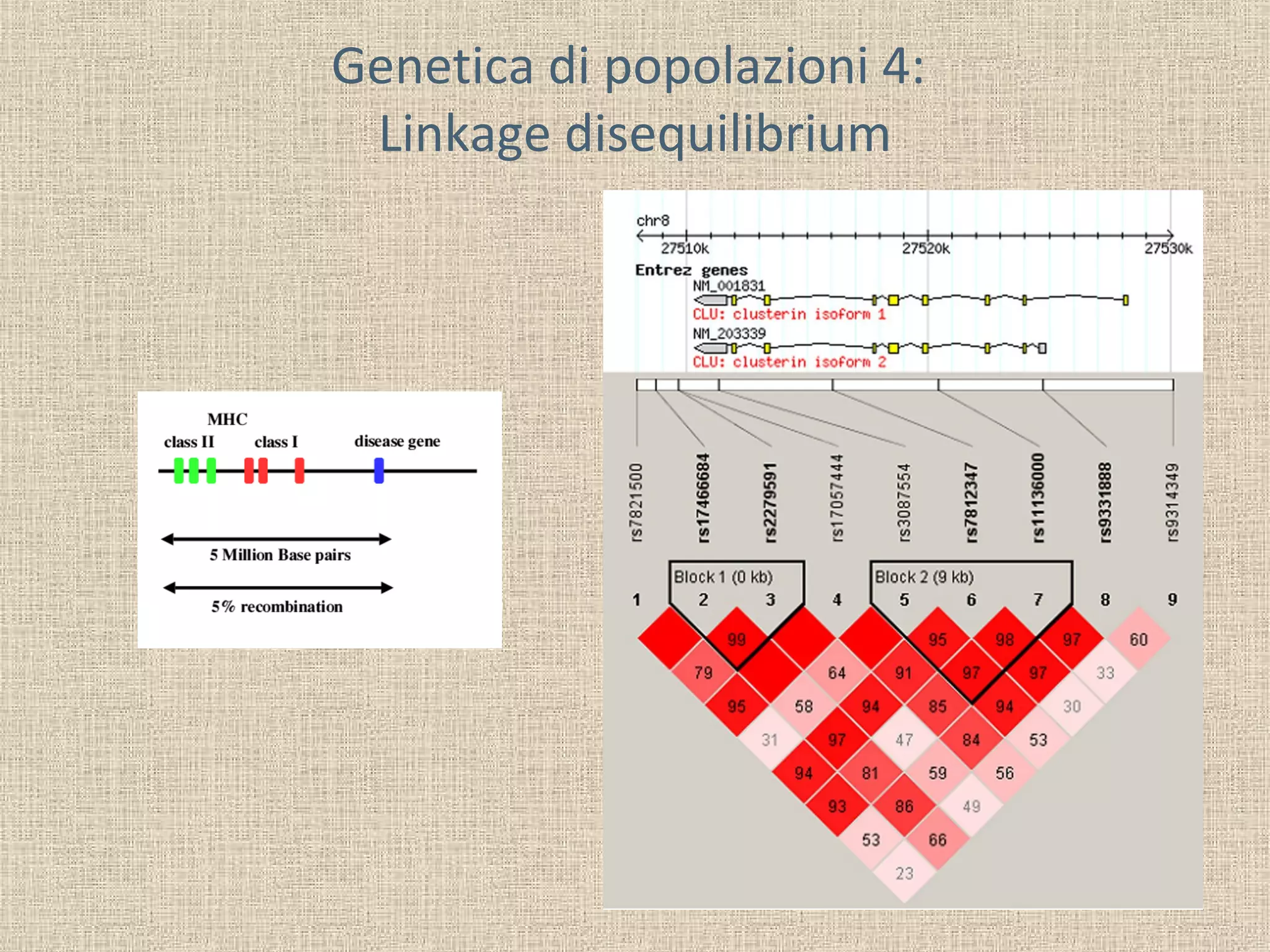
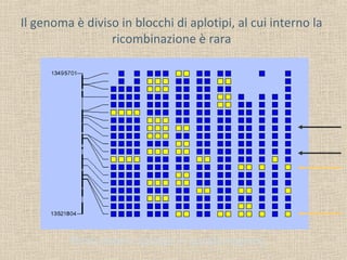
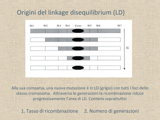
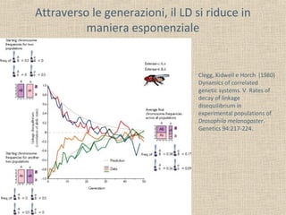
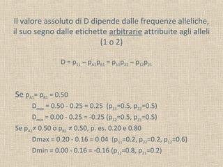
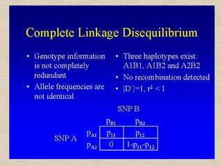
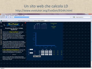
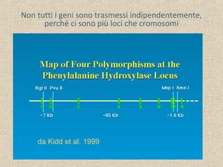
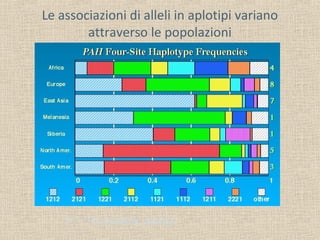
Il documento tratta della genetica di popolazioni, focalizzandosi sul linkage disequilibrium (LD) e i suoi fondamenti, come l'equilibrio di Hardy-Weinberg, la mutazione e la ricombinazione. Descrive come il LD e la sua riduzione nel tempo dipendano dai tassi di ricombinazione e dal numero di generazioni, sottolineando l'importanza dei aplotipi. Inoltre, evidenzia che, mentre l'equilibrio di Hardy-Weinberg può essere raggiunto rapidamente, il linkage equilibrium richiede più tempo e può essere analizzato tramite diverse statistiche.

1. Genetica di popolazioni 4:
Linkage disequilibrium

2. Programma del corso
1. Diversità genetica
2. Equilibrio di Hardy-Weinberg
3. Inbreeding
4. Linkage disequilibrium
5. Mutazione
6. Deriva genetica
7. Flusso genico e varianze genetiche
8. Selezione
9. Mantenimento dei polimorfismi e teoria neutrale
10. Introduzione alla teoria coalescente
11. Struttura e storia della popolazione umana
+ Lettura critica di articoli

3. Linkage e linkage disequilibrium
Linkage: l’associazione fisica dei loci sui cromosomi,
Linkage disequilibrium: l’associazione non casuale degli alleli
di diversi loci nei cromosomi/gameti, a formare aplotipi.
Il linkage è una causa (non la sola) del linkage disequilibrum

4. Equilibrio e disequilibrio
pB1
pB2
pB1
pA1
pA1
pA2
pA2
pB2

5. Il genoma è diviso in blocchi di aplotipi, al cui interno la
ricombinazione è rara
Nove diversi aplotipi in questa regione

6. Origini del linkage disequilibrium (LD)
Alla sua comparsa, una nuova mutazione è in LD (grigio) con tutti I loci dello
stesso cromosoma. Attraverso le generazioni la ricombinazione riduce
progressivamente l’area di LD. Contano soprattutto:
1. Tasso di ricombinazione
2. Numero di generazioni

7. Quindi: Equilibrio di Hardy-Weinberg e
linkage disequilibrium
• Basta una generazione di accoppiamento casuale per
raggiungere l’equilibrio di HW a un locus
• Se si studiano più loci, possono essere necessarie
parecchie generazioni perché si raggiunga anche un
linkage equilibrium, cioé perché gli alleli siano associati
casualmente nei gameti

8. Attraverso le generazioni, il LD si riduce in
maniera esponenziale
cromosomi in LD
ricombinazione
cromosomi con assoc.
casuale degli alleli
r
(1-r)
non ricombinazione
cromosomi in LD
LD fra due loci al tempo t: Dt = (1-r)t D0

9. Attraverso le generazioni, il LD si riduce in
maniera esponenziale
Clegg, Kidwell e Horch (1980)
Dynamics of correlated
genetic systems. V. Rates of
decay of linkage
disequilibrium in
experimental populations of
Drosophila melanogaster.
Genetics 94:217-224.

10. Vediamo se ci siamo capiti
Perché il LD declina più
rapidamente del
previsto?
Perché nell’esperimento
indicato dalla linea blu
alla fine si ottiene un LD
opposto a quello di
partenza?

11. E attraverso le generazioni si riduce anche
l’area di LD
Nature Reviews Genetics 4; 701-709 (2003)

12. Se gli alleli ai due loci non sono associati in maniera casuale,
ci sarà una deviazione delle frequenze degli aplotipi (D)
rispetto alle frequenze attese:
p11 = p1q1 + D
p12 = p1q2 – D
p21 = p2q1 – D
p22 = p2q2 + D
Il parametro D è il coefficiente di linkage disequilibrium,
proposto per primi da Lewontin e Kojima (1960).
Dmax è uguale a min (p1q2, p2q1) per D>0,
o a max (-p1q1, -p2q2) per D < 0.

14. Il valore assoluto di D dipende dalle frequenze alleliche,
il suo segno dalle etichette arbitrarie attribuite agli alleli
(1 o 2)
D = p11 – pA1pB1 = p11p22 – p12p21
Se pA1= pB1 = 0.50
Dmax = 0.50 - 0.25 = 0.25 (p11=0.5, p22=0.5)
Dmin = 0.00 - 0.25 = -0.25 (p12=0.5, p21=0.5)
Se pA1≠ 0.50 o pB1 ≠ 0.50, p. es. 0.20 e 0.80
Dmax = 0.20 - 0.16 = 0.04 (p11=0.2, p22=0.2, p12=0.6)
Dmin = 0.00 - 0.16 = -0.16 (p12=0.8, p21=0.2)

19. Un sito web che calcola LD
http://www.evotutor.org/EvoGen/EG4A.html

20. Non tutti i geni sono trasmessi indipendentemente,
perché ci sono più loci che cromosomi
da Kidd et al. 1999

21. Le associazioni di alleli in aplotipi variano
attraverso le popolazioni
24 = 16 possibili aplotipi

22. I livelli di linkage disequilibrium variano
attraverso le popolazioni

23. Arabidopsis, Nordborg et al. 2005

24. Solo una frazione degli aplotipi possibili è presente
nelle popolazioni
Crawford et al. 2004

25. Ma una larga parte degli aplotipi presenti è
condivisa fra popolazioni
Una media di 5.3 blocchi di
aplotipi per ogni regione di
genoma (15 Mb
complessivamente)

26. Rappresentazione
grafica del linkage
disequilibrium e
individuazione di
blocchi
SNP associati con una forma
di schizofrenia (parte alta del
grafico) e
blocchi di LD (in rosso, in
basso) attraverso 209 kb.
Shi et al. (2009) Common
variants on chromosome
6p22.1 are associated with
schizophrenia. Nature 460:
753-757

27. Una review non recentissima, ma ancora buona

28. Sintesi
• Due loci sono in linkage equilibrium se le frequenze
genotipiche a un locus sono indipendenti da quelle all’altro
locus
• Il linkage disequilibrium è causato dalla mutazione e ridotto
dalla ricombinazione
• Basta una generazione di accoppiamento casuale per
raggiungere l’equilibrio di Hardy-Weinberg, ma non il LD
• Si misura il LD confrontando frequenze genotipiche
osservate e attese a due loci, tramite le statistiche r, D e D’