Downloaded 61 times


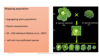
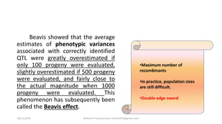
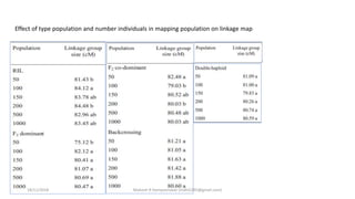
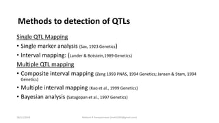
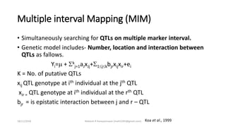
![• Population permits the visualization of F1 gametes – test cross, BC and
double haploids
• F2 and F2:3 – maximum like methods, Importance Sampling Methods
and Genealogy Methods
• RILs first calculate the R r = R/[2(1-r)]
18/11/2018 Mahesh R Hampannavar (mahi5295@gmail.com)](https://image.slidesharecdn.com/seminar-2-181118161151/85/Quantitative-Trait-LOci-QTLs-Mapping-Basics-procedure-principle-and-Methods-26-320.jpg)
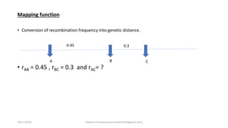
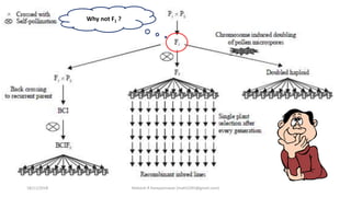
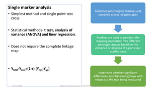
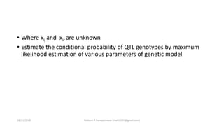
![The Haldane Distance
• rAC = rAB + rBC
• But multiple crossing over
tend to reduce the
recombination rate between
the genes.
• rAC = rAB + rBC – 2rAB*rBC
• m = -50ln(1-2r)
Kosambi Mapping function
• rAC = rAB + rBC
• multiple crossing over tend to
reduce the recombination rate
between the genes.
• Interference
• Coincidence (denoted by ‘c’)
• rAC = rAB + rBC – 2crAB*rBC
• mk= 25ln[(1+2r)/(1-2r)]
18/11/2018 Mahesh R Hampannavar (mahi5295@gmail.com)](https://image.slidesharecdn.com/seminar-2-181118161151/85/Quantitative-Trait-LOci-QTLs-Mapping-Basics-procedure-principle-and-Methods-30-320.jpg)
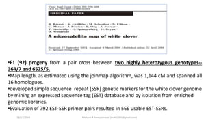
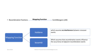
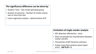
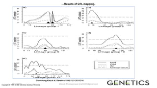
![AABB X aabb
AaBb X aabb
AaBb, Aabb, aaBb, aabb
9 : 1 : 1 : 9
LOD score (z) = log10 [r(1- )n-r/0.5 n ]
LOD SCORE CALCULATION
18/11/2018 Mahesh R Hampannavar (mahi5295@gmail.com)](https://image.slidesharecdn.com/seminar-2-181118161151/85/Quantitative-Trait-LOci-QTLs-Mapping-Basics-procedure-principle-and-Methods-32-320.jpg)
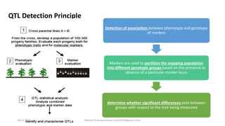
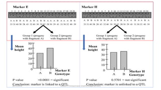
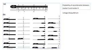

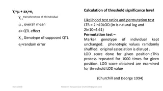
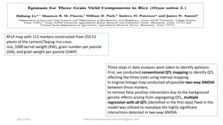
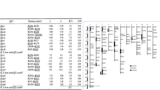
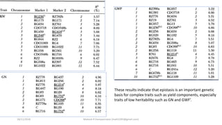


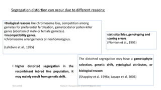
The document discusses strategies for identifying quantitative trait loci (QTL) and trait introgression, highlighting the importance of constructing linkage maps and using genetic markers for marker-assisted selection. It explains the mapping population, methods for detecting QTLs, including single-marker and composite interval mapping, and the significance of factors such as population size and statistical methods in QTL analysis. Additionally, it addresses limitations of various QTL detection methods and emphasizes the need for appropriate software and methodologies for effective genetic mapping.


