The document discusses Gauss-Seidel, Successive Over Relaxation (SOR), and block SOR methods for solving systems of linear equations. Gauss-Seidel converges faster than Jacobi iteration. SOR can further accelerate convergence by introducing a relaxation parameter ω between 0 and 2. Block SOR generalizes the approach to block-structured matrices by solving blocks simultaneously. Examples show how to apply these methods to finite difference discretizations in 2D and 3D.

1. 5.2 Gauss-Seidel and SOR (Successive Over Relaxation)
As motivation return to the example of the last section:
−ui −1 + 3ui −ui +1 = f i .
Jacobi: uim +1 = ( f i + uim 1 + uim 1 ) / 3
− + i = 1,2,...,n.
Since ui-1 m+1 has already been computed and may be closer to the solution, we should
consider using it in place of ui-1 m. This is the Gauss-Seidel method
Gauss-Seidel: uim +1 = ( f i + uim 1 1 + uim 1 ) / 3
−
+
+ i = 1,2,...,n.
For the Gauss-Seidel scheme and the given example, the iterates one and two are
0   1/3   13/27 
0  , u1 =  4 / 9  and u 2 =  53/81  .
u = 
0
   
0 
  13/27 
  124/243 
 
Gauss-Seidel exhibits faster convergence.
SOR Algorithm (0 < ω < 2)
Note, ω = 1.0 is Gauss-Seidel, ω > 1.0 is over-relaxation, and ω < 1.0 is
under-relaxation. Consider Ax = d or in component form
∑a
j< i
i, j x j + ai ,i xi + ∑ ai , j x j = di .
j> i
for m = 0, maxm
for i = 1, n
xim +1 / 2 = ( di − ∑ ai , j x m +1 − ∑ ai , j x m ) / ai , i
j j
j< i j >i
xim +1 = (1 − ω ) xim + ω xim +1 / 2
test for convergence.

2. 2
Most applications are sparse (many aij = 0). Gauss-Seidel would not be used on
dense matrices because of the number of calculations required for the lower and upper
sums.
Notes: (i) If A SPD and 0 < ω < 2, then we will show that SOR converges.
(ii) ω > 1.0 is used to significantly accelerate convergence
(The choice of ω could be a problem for some application).
(iii) ω =1.0 (for G-S) is much faster than Jacobi.
SOR may be viewed as a matrix FOFD iteration
* 0 0 0  0 0 0 0  0 * * *
0 * 0 0  * 0 0 0  0 0 * *
A = D − L −U =  −  −  
0 0 * 0  * * 0 0  0 0 0 *
     
0 0 0 *  * * * 0  0 0 0 0
Then xim +1 = (1 − ω ) xim + ω (di − ∑ ai , j x m +1 −∑ ai , j x m ) / ai ,i
j j
j <i j >i
a x m +1
i, i i = (1 − ω )a x + ω (di − ∑ ai , j x m +1 −∑ ai , j x m )
m
i, i i j j
j <i j >i
The matrix form is
Dx m +1 = (1− ω ) Dx m + ω (d + Lxm +1 + Ux m )
( D − ω L) x m +1 = (1 − ω ) Dx m + ωUx m + ω d
( D − ω L ) x m +1 / ω = (1 − ω) Dx m / ω + Ux m + d
x m +1 = [( D − ω L) / ω] −1[(1 − ω ) D / ω + U ] x m + [( D − ω L) / ω ]−1 d
x m +1 = Hω x m + [( D − ω L ) / ω ]−1 d

3. 3
We need || Hω || < 1 to qualify as a convergent FOFD. Moreover, we want ϖ such that
|| Hϖ || ≤ || Hω || so that the convergence will be fast.
Example. Two dimensional, point SOR for -∆u = f.
Unknowns are uij ≅ u(ih,jh) h = ∆x = ∆y.
Use the five point finite difference method:
−ui −1, j −ui , j −1 + 4ui , j −ui +1, j − ui , j +1 = h 2 f i , j .
(lower sum + ai,i xi + upper sum)
In order to cast this problem in the form of Ax = d, make the following
identifications:
i → i,j pair ,
xi → ui,j ,
ai,i = 4 ,
aij = -1 for j identified with the grid pairs (i+1,j), (i-1,j),(i,j+1) and (i,j-1),
n → (N-1)2 and
d → h2 fi,j with h = 1/N.
The classical order of nodes starts with the bottom grid row (j = 1) and moves
from left (i = 1) to the right (i = N-1)
 
 # # # 
 
lower↓  * i, j #  ↑upper
 
 * * * 

 


4. 4
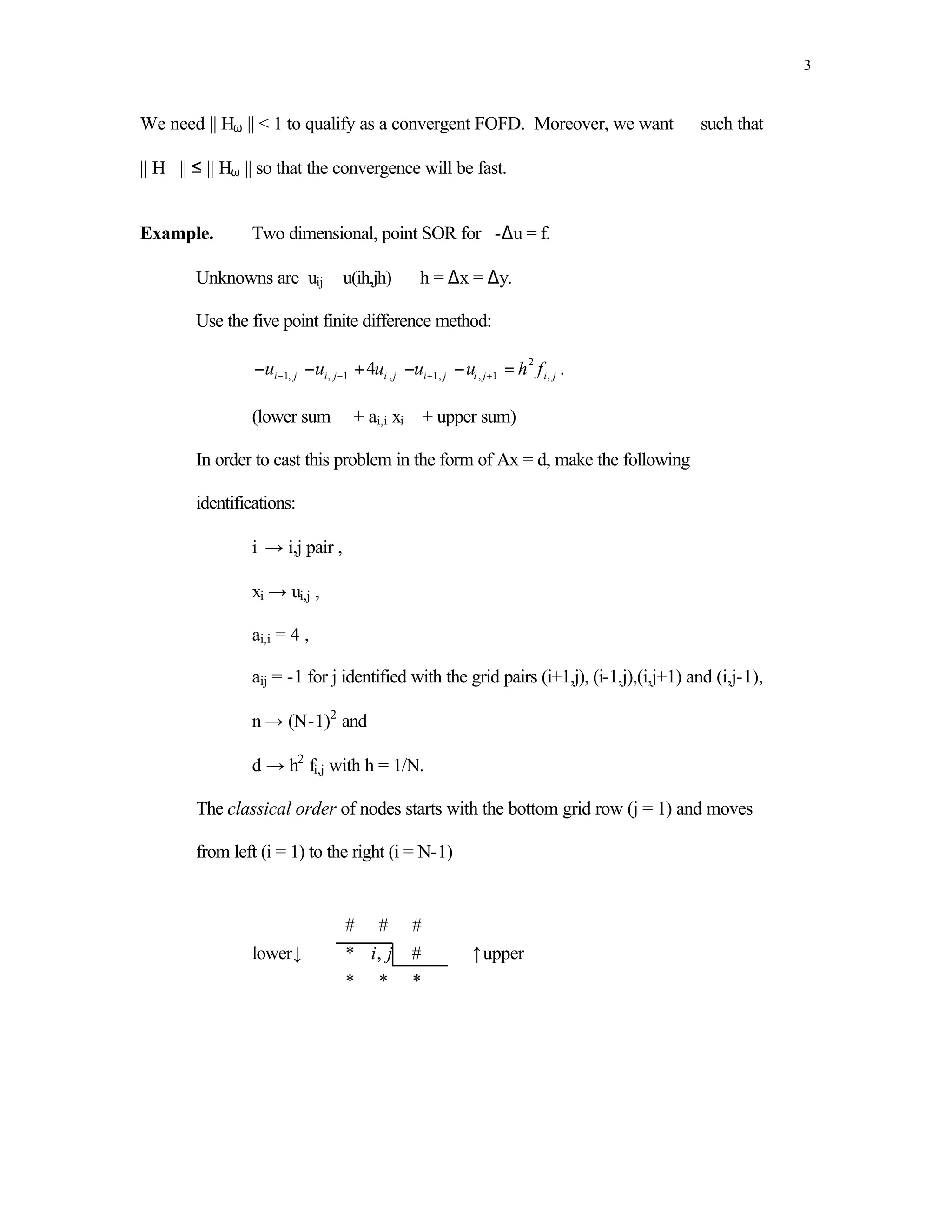
Point SOR with u(i,j) Overwritten.
for m = 0, maxm
numi = 0
for j = 1, N-1
for i = 1, N-1
utemp = [h*h*fij +u(i-1,j)+u(i,j-1)+u(i+1,j)+u(i,j+1)]*0.25
utemp = (1-ω)*u(i,j) + ω*utemp
error = u(i,j) - utemp
if abs(error) < ε numi = numi + 1
u(i,j) = utemp
if numi = (N-1)*(N-1) break
See MA402 chapters 3,4 for MATLAB and Fortran 90 implementations.
Example. Two dimensional block SOR.
B −I   U1   F1 
A =  −I   U  = h2  F 
 B −I  2   2

 −I B  U 3 
   F3 
 
 4 −1   u11 
 −1 4 −1 ,
B =  U1 =  u21  ,
  I3x3

 −1 4 
  u31 
 
−U i −1 + BU i − U i +1 = h 2 Fi .
Here i represents the i grid row (an abuse of notation)
Block component form iss A = [Aij] where A is (N-1)x(N-1) block matrix.

5. 5
AX = F
∑A X
j< i
ij j + Aii X i + ∑ Aij X j = Fi where Aii are tridiagonal matrices.
j> i
Block G-S algorithm.
for m = 1, maxm
for i = 1,N-1
Solve Aii X im +1 = Fi − ∑ Aij X m +1 − ∑ Aij X m
j j
j< i j> i
test for convergence.
Example. Three dimensional point SOR for -∆u = f.
This is similar to the 2D point SOR with an additional loop in z direction.
The 7 point finite difference equation is
−ui −1, j , l −ui , j− 1,l −ui , j ,l −1 + 6ui , j ,l −ui +1, j ,l − ui , j+ 1,l − ui , j ,l + 1 = h 2 f i ,j ,l .
The point SOR scheme will now have three inner nested loops. The coefficient
matrix will be block tridiagonal with the diagonal blocks having a similar
structure as the 2D coefficient matrix.